Python & OpenGL for Scientific Visualization
Copyright (c) 2018 - Nicolas P. Rougier <Nicolas.Rougier@inria.fr>


Preface
.
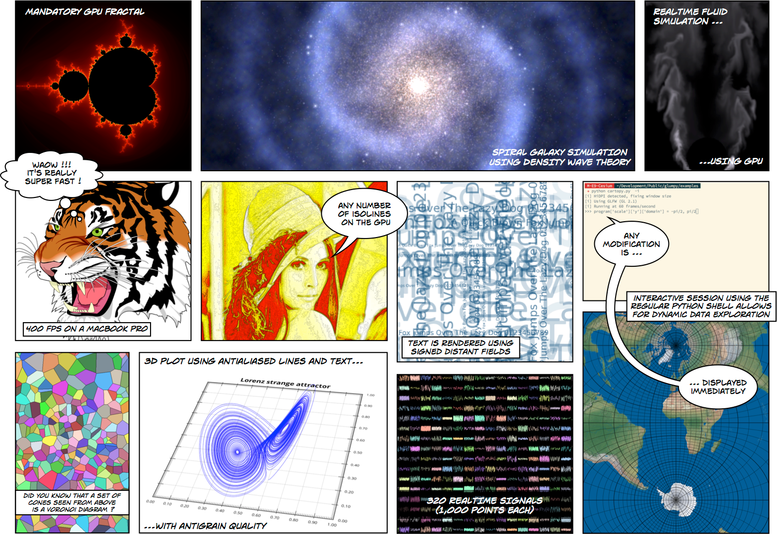
This book is open-access (i.e. it's free to read at this address) because I believe knowledge should be free. However, if you think the book is worth a few dollars, you can give me a few euros (5€ or 10€). This money will help me to travel to Python conferences and to write other books as well. If you don't have money, it's fine. Just enjoy the book and spread the word about it. The teaser image above comes from the artwork section of my website. It has been made some years ago using the Povray (Persistence of Vision) raytracer. I like it very much because it is a kind of résumé of my research.
About the author
I am a full-time research scientist at Inria which is the French national institute for research in computer science and control. This is a public scientific and technological establishment (EPST) under the double supervision of the Research & Education Ministry, and the Ministry of Economy Finance and Industry. I'm working within the Mnemosyne project which lies at the frontier between integrative and computational neuroscience in association with the Institute of Neurodegenerative Diseases, the Bordeaux laboratory for research in computer science (LaBRI), the University of Bordeaux and the national center for scientific research (CNRS).
I've been using Python for more than 15 years and numpy for more than 10 years for modeling in neuroscience, machine learning and for advanced visualization (OpenGL). I'm the author of several online resources and tutorials (Matplotlib, numpy, OpenGL) and I've been teaching Python, numpy and scientific visualization at the University of Bordeaux and in various conferences and schools worldwide (SciPy, EuroScipy, etc). I'm also the author of the popular article Ten Simple Rules for Better Figures , a popular matplotlib tutorial and an open access book From Python To Numpy.
About this book
This book has been written in restructured text format and generated using a customized version of the docutils rst2html.py command line (available from the docutils python package) and a custom template.
If you want to rebuild the html output, from the top directory, type:
$ ./rst2html.py --link-stylesheet            \
                --cloak-email-addresses      \
                --toc-top-backlinks          \
                --stylesheet book.css        \
                --stylesheet-dirs .          \
                book.rst book.html
Or you use the provided make.sh shell script.
The sources are available from https://github.com/rougier/python-opengl.
Last point, I wrote the book in a kind of modern Kerouac's style such that you can download it once and continue reading it offline. Initial loading may be slow though.
Prerequisites
This is not a Python nor a NumpPy beginner guide and you should have an intermediate level in both Python and NumPy. No prior knowledge of OpenGL is necessary because I'll explain everything.
Conventions
I will use usual naming conventions. If not stated explicitly, each script should import numpy, scipy and glumpy as:
import numpy as np
We'll use up-to-date versions (at the date of writing, i.e. August, 2017) of the different packages:
| Packages | Version |
|---|---|
| Python | 3.6.0 |
| Numpy | 1.12.0 |
| Scipy | 0.18.1 |
| Cython | 0.25.2 |
| Triangle | 20170106 |
| Glumpy | 1.0.6 |
How to contribute
If you want to contribute to this book, you can:
- Report issues (https://github.com/rougier/python-opengl/issues)
- Suggest improvements (https://github.com/rougier/python-opengl/pulls)
- Correct English (https://github.com/rougier/python-opengl/issues)
- Star the project (https://github.com/rougier/python-opengl)
- Suggest a more responsive design for the HTML Book
- Spread the word about this book (Reddit, Hacker News, etc.)
Publishing
If you're an editor interested in publishing this book, you can contact me if you agree to have this version and all subsequent versions open access (i.e. online at this address), you know how to deal with restructured text (Word is not an option), you provide a real added-value as well as supporting services, and more importantly, you have a truly amazing latex book template (and be warned that I'm a bit picky about typography & design: Edward Tufte is my hero). Still here?
License
Book
This work is licensed under a Creative Commons Attribution-Non Commercial-Share Alike 4.0 International License. You are free to:
- Share — copy and redistribute the material in any medium or format
- Adapt — remix, transform, and build upon the material
The licensor cannot revoke these freedoms as long as you follow the license terms.
Under the following terms:
- Attribution — You must give appropriate credit, provide a link to the license, and indicate if changes were made. You may do so in any reasonable manner, but not in any way that suggests the licensor endorses you or your use.
- NonCommercial — You may not use the material for commercial purposes.
- ShareAlike — If you remix, transform, or build upon the material, you must distribute your contributions under the same license as the original.
Code
The code is licensed under the OSI-approved BSD 2-Clause License.
Introduction
.
Before diving into OpenGL programming, it is important to have a look at the whole GL landscape because it is actually quite complex and you can easily lose yourself between the different actors, terms and definitions. The teaser image above shows the face of a character from the Wolfenstein game, one from 1992 and the other from 2015. You can see that computer graphics has evolved a lot in 25 years.
A bit of history
OpenGL is 25 years old! Since the first release in 1992, a lot has happened (and is still happening actually, with the newly released Vulkan API and the 4.6 GL release) and consequently, before diving into the book, it is important to understand OpenGL API evolution over the years. If the first API (1.xx) has not changed too much in the first twelve years, a big change occurred in 2004 with the introduction of the dynamic pipeline (OpenGL 2.x), i.e. the use of shaders that allow to have direct access to the GPU. Before this version, OpenGL was using a fixed pipeline that made it easy to rapidly prototype some ideas. It was simple but not very powerful because the user had not much control over the graphic pipeline. This is the reason why it has been deprecated more than ten years ago and you don't want to use it today. Problem is that there are a lot of tutorials online that still use this fixed pipeline and because most of them were written before modern GL, they're not even aware (and cannot) that they use a deprecated API.
How to know if a tutorial address the fixed pipeline ? It's relatively easy. It'll contain GL commands such as:
glVertex, glColor, glLight, glMaterial, glBegin, glEnd, glMatrix,
glMatrixMode, glLoadIdentity, glPushMatrix, glPopMatrix, glRect,
glPolygonMode, glBitmap, glAphaFunc, glNewList, glDisplayList,
glPushAttrib, glPopAttrib, glVertexPointer, glColorPointer,
glTexCoordPointer, glNormalPointer, glRotate, glTranslate, glScale,
glMatrixMode, glCall,
If you see any of them in a tutorial, run away because it it's most certainly a tutorial that address the fixed pipeline and you don't want to read it because what you will learn is already useless. If you look at the GL history below, you'll realize that the "modern" GL API is already 13 years old while the fixed pipeline has been deprecated more than 10 years ago.
 1                       2         Modern              2
 9                       0         OpenGL              0               Vulkan
 9                       0           ↓                 1                 ↓
 2  3  4  5  6  7  8  9  0  1  2  3  4  5  6  7  8  9  0  1  2  3  4  5  6  7
─────────────────────────────────────┬───────────────────────────────────┬────
OpenGL                                                3.3
                                                      4.0
                                                   3.1
                  1.2         1.4   2.0            3.2   4.2   4.4
1.0            1.1         1.3   1.5      2.1   3.0   4.1   4.3   4.5      4.6
╌╌╌╌╌╌╌╌╌╌╌╌╌╌╌╌╌╌╌╌╌╌╌╌╌╌╌╌╌╌╌╌╌╌╌╌╌┬╌╌╌╌╌╌╌╌╌╌╌╌╌╌╌╌╌╌╌╌╌╌╌╌╌╌╌╌╌╌╌╌╌╌╌╌╌╌╌╌
           Fixed pipeline            ╎           Programmable pipeline
╌╌╌╌╌╌╌╌╌╌╌╌╌╌╌╌╌╌╌╌╌╌╌╌╌╌╌╌╌╌╌╌╌╌╌╌╌┴╌╌╌╌╌╌╌╌╌╌╌╌╌╌╌╌╌╌╌╌╌╌╌╌╌╌╌╌╌╌╌╌╌╌╌╌╌╌╌╌
GLES                                    ╭─────╮                      3.2
                              1.0       │ 2.0 │             3.0   3.1
                                        ╰─────╯
╌╌╌╌╌╌╌╌╌╌╌╌╌╌╌╌╌╌╌╌╌╌╌╌╌╌╌╌╌╌╌╌╌╌╌╌╌╌╌╌╌╌╌╌╌╌╌╌╌╌╌╌╌╌╌╌╌╌╌╌╌╌╌╌╌╌╌╌╌╌╌╌╌╌╌╌╌╌
GLSL                                                  4.0   4.3   4.5      4.6
                                                1.3   4.1      4.4
                                                   1.4   4.2
                                    1.1   1.2      1.5
╌╌╌╌╌╌╌╌╌╌╌╌╌╌╌╌╌╌╌╌╌╌╌╌╌╌╌╌╌╌╌╌╌╌╌╌╌╌╌╌╌╌╌╌╌╌╌╌╌╌╌╌╌╌╌╌╌╌╌╌╌╌╌╌╌╌╌╌╌╌╌╌╌╌╌╌╌╌
WebGL                                             1.0                      2.0
╌╌╌╌╌╌╌╌╌╌╌╌╌╌╌╌╌╌╌╌╌╌╌╌╌╌╌╌╌╌╌╌╌╌╌╌╌╌╌╌╌╌╌╌╌╌╌╌╌╌╌╌╌╌╌╌╌╌╌╌╌╌╌╌╌╌╌╌╌╌╌╌╌╌╌╌╌╌
Vulkan                                                                  1.0
──────────────────────────────────────────────────────────────────────────────
From OpenGL wiki: In 1992, Mark Segal and Kurt Akeley authored the OpenGL 1.0 specification which formalized a graphics API and made cross platform 3rd party implementation and support viable. In 2004, OpenGL 2.0 incorporated the significant addition of the OpenGL Shading Language (also called GLSL), a C like language with which the transformation and fragment shading stages of the pipeline can be programmed. In 2008, OpenGL 3.0 added the concept of deprecation: marking certain features as subject to removal in later versions.
- Open Graphics Library (OpenGL)
- OpenGL is a cross-language, cross-platform application programming interface (API) for rendering 2D and 3D vector graphics. The API is typically used to interact with a graphics processing unit (GPU), to achieve hardware-accelerated rendering.
- OpenGL for Embedded Systems (OpenGL ES or GLES)
- GLES is a subset of the OpenGL computer graphics rendering application programming interface (API) for rendering 2D and 3D computer graphics such as those used by video games, typically hardware-accelerated using a graphics processing unit (GPU).
- OpenGL Shading Language (GLSL)
- GLSL is a high-level shading language with a syntax based on the C programming language. It was created by the OpenGL ARB (OpenGL Architecture Review Board) to give developers more direct control of the graphics pipeline
- Web Graphics Library (WebGL)
- WebGL is a JavaScript API for rendering 3D graphics within any compatible web browser without the use of plug-ins. WebGL is integrated completely into all the web standards of the browser allowing GPU accelerated usage of physics and image processing and effects as part of the web page canvas.
- Vulkan (VK)
- Vulkan is a low-overhead, cross-platform 3D graphics and compute API first announced at GDC 2015 by the Khronos Group. Like OpenGL, Vulkan targets high-performance realtime 3D graphics applications such as video games and interactive media across all platforms, and can offer higher performance and more balanced CPU/GPU usage, much like Direct3D 12 and Mantle.
For this book, we'll use the GLES 2.0 API that allows to use the modern GL API while staying relatively simple. For comparison, have a look at the table below that gives the number of functions and constants for each version of the GL API. Note that once you'll master the GLES 2.0, it's only a matter of reading the documentation to take advantage of more advanced version because the core concepts remain the same (which is not the case for the new Vulkan API).
Note
The number of functions and constants have been computed using the code/chapter-02/registry.py program that parses the gl.xml file that defines the OpenGL and OpenGL API Registry
| Version | Constants | Functions | Version | Constants | Functions | |
|---|---|---|---|---|---|---|
| GL 1.0 | 0 | 306 | GL 3.2 | 800 | 316 | |
| GL 1.1 | 528 | 336 | GL 3.3 | 816 | 344 | |
| GL 1.2 | 569 | 340 | GL 4.0 | 894 | 390 | |
| GL 1.3 | 665 | 386 | GL 4.1 | 929 | 478 | |
| GL 1.4 | 713 | 433 | GL 4.2 | 1041 | 490 | |
| GL 1.5 | 763 | 452 | GL 4.3 | 1302 | 534 | |
| GL 2.0 | 847 | 545 | GL 4.4 | 1321 | 543 | |
| GL 2.1 | 870 | 551 | GL 4.5 | 1343 | 653 | |
| GL 3.0 | 1104 | 635 | GLES 1.0 | 333 | 106 | |
| GL 3.1 | 1165 | 647 | GLES 2.0 | 301 | 142 |
Modern OpenGL
The graphic pipeline
Note
The shader language is called glsl. There are many versions that goes from 1.0 to 1.5 and subsequent version get the number of OpenGL version. Last version is 4.6 (June 2017).
If you want to understand modern OpenGL, you have to understand the graphic pipeline and shaders. Shaders are pieces of program (using a C-like language) that are build onto the GPU and executed during the rendering pipeline. Depending on the nature of the shaders (there are many types depending on the version of OpenGL you're using), they will act at different stage of the rendering pipeline. To simplify this tutorial, we'll use only vertex and fragment shaders as shown below:
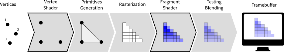
A vertex shader acts on vertices and is supposed to output the vertex
position (gl_Position) on the viewport (i.e. screen). A fragment shader
acts at the fragment level and is supposed to output the color
(gl_FragColor) of the fragment. Hence, a minimal vertex shader is:
void main()
{
    gl_Position = vec4(0.0,0.0,0.0,1.0);
}
while a minimal fragment shader would be:
void main()
{
    gl_FragColor = vec4(0.0,0.0,0.0,1.0);
}
These two shaders are not very useful because the first shader will always
output the null vertex (gl_Position is a special variable) while the second
will only output the black color for any fragment (gl_FragColor is also a
special variable). We'll see later how to make them to do more useful things.
One question remains: when are those shaders executed exactly ? The vertex shader is executed for each vertex that is given to the rendering pipeline (we'll see what does that mean exactly later) and the fragment shader is executed on each fragment (= pixel) that is generated after the vertex stage. For example, in the simple figure above, the vertex would be called 3 times, once for each vertex (1,2 and 3) while the fragment shader would be executed 21 times, once for each fragment.
Buffers
The next question is thus where do those vertices comes from ? The idea of modern GL is that vertices are stored on the CPU and need to be uploaded to the GPU before rendering. The way to do that is to build buffers onto the CPU and to send these buffers onto the GPU. If your data does not change, no need to upload them again. That is the big difference with the previous fixed pipeline where data were uploaded at each rendering call (only display lists were built into GPU memory).
But what is the structure of a vertex ? OpenGL does not assume anything about your vertex structure and you're free to use as many information you may need for each vertex. The only condition is that all vertices from a buffer have the same structure (possibly with different content). This again is a big difference with the fixed pipeline where OpenGL was doing a lot of complex rendering stuff for you (projections, lighting, normals, etc.) with an implicit fixed vertex structure. The good news is that you're now free to do anything you want, but the bad news is that you have to program just everything.
Let's take a simple example of a vertex structure where we want each vertex to hold a position and a color. The easiest way to do that in python is to use a structured array using numpy:
data = np.zeros(4, dtype = [ ("position", np.float32, 3),
                             ("color",    np.float32, 4)] )
We just created a CPU buffer with 4 vertices, each of them having a
position (3 floats for x,y,z coordinates) and a color (4 floats for
red, blue, green and alpha channels). Note that we explicitly chose to have 3
coordinates for position but we may have chosen to have only 2 if were to
work in two-dimensions. Same holds true for color. We could have used
only 3 channels (r,g,b) if we did not want to use transparency. This would save
some bytes for each vertex. Of course, for 4 vertices, this does not really
matter but you have to realize it will matter if your data size grows up to
one or ten million vertices.
Variables
Now, we need to explain our shaders what to do with these buffers and how to connect them together. So, let's consider again a CPU buffer of 4 vertices using 2 floats for position and 4 floats for color:
data = np.zeros(4, dtype = [ ("position", np.float32, 2),
                             ("color",    np.float32, 4)] )
We need to tell the vertex shader that it will have to handle vertices where a position is a tuple of 2 floats and color is a tuple of 4 floats. This is precisely what attributes are meant for. Let us change slightly our previous vertex shader:
attribute vec2 position;
attribute vec4 color;
void main()
{
    gl_Position = vec4(position, 0.0, 1.0);
}
This vertex shader now expects a vertex to possess 2 attributes, one named
position and one named color with specified types (vec2 means tuple of
2 floats and vec4 means tuple of 4 floats). It is important to note that even
if we labeled the first attribute position, this attribute is not yet bound
to the actual position in the numpy array. We'll need to do it explicitly
at some point in our program and there is no magic that will bind the numpy
array field to the right attribute, you'll have to do it yourself, but we'll
see that later.
The second type of information we can feed the vertex shader is the uniform
that may be considered as constant value (across all the vertices). Let's say
for example we want to scale all the vertices by a constant factor scale,
we would thus write:
uniform float scale;
attribute vec2 position;
attribute vec4 color;
void main()
{
    gl_Position = vec4(position*scale, 0.0, 1.0);
}
Last type is the varying type that is used to pass information between the vertex stage and the fragment stage. So let us suppose (again) we want to pass the vertex color to the fragment shader, we now write:
uniform float scale;
attribute vec2 position;
attribute vec4 color;
varying vec4 v_color;

void main()
{
    gl_Position = vec4(position*scale, 0.0, 1.0);
    v_color = color;
}
and then in the fragment shader, we write:
varying vec4 v_color;

void main()
{
    gl_FragColor = v_color;
}
The question is what is the value of v_color inside the fragment shader ?
If you look at the figure that introduced the gl pipeline, we have 3 vertices
and 21 fragments. What is the color of each individual fragment ?
The answer is the interpolation of all 3 vertices color. This interpolation is made using the distance of the fragment to each individual vertex. This is a very important concept to understand. Any varying value is interpolated between the vertices that compose the elementary item (mostly, line or triangle).
Ok, enough for now, we'll see an explicit example in the next chapter.
State of the union
Last, but not least, we need to access the OpenGL library from within Python and we have mostly two solutions at our disposal. Either we use pure bindings and we have to program everything (see next chapter) or we use an engine that provide a lot of convenient functions that ease the development. We'll first use the PyOpenGL bindings before using the glumpy library that offers a tight integration with numpy.
Bindings
- Pyglet is a pure python cross-platform application framework intended for game development. It supports windowing, user interface event handling, OpenGL graphics, loading images and videos and playing sounds and music. It works on Windows, OS X and Linux.
- PyOpenGL is the most common cross platform Python binding to OpenGL and related APIs. The binding is created using the standard ctypes library, and is provided under an extremely liberal BSD-style Open-Source license.
- ModernGL is a wrapper over OpenGL that simplifies the creation of simple graphics applications like scientific simulations, small games or user interfaces. Usually, acquiring in-depth knowledge of OpenGL requires a steep learning curve. In contrast, ModernGL is easy to learn and use, moreover it is capable of rendering with the same performance and quality, with less code written.
- Ctypes bindings can also be generated quite easily thanks to the gl.xml file provided by the Khronos group that defines the OpenGL and OpenGL API Registry. The number of functions and constants given in the table above have been computed using the code/chapter-02/registry.py program that parses the gl.xml file for each API and version and count the relevant features.
Engines
- The Visualization Toolkit (VTK) is an open-source, freely available software system for 3D computer graphics, image processing, and visualization. It consists of a C++ class library and several interpreted interface layers including Tcl/Tk, Java, and Python.
- Processing is a programming language, development environment, and online community. Since 2001, Processing has promoted software literacy within the visual arts and visual literacy within technology. Today, there are tens of thousands of students, artists, designers, researchers, and hobbyists who use Processing for learning, prototyping, and production.
- NodeBox for OpenGL is a free, cross-platform library for generating 2D animations with Python programming code. It is built on Pyglet and adopts the drawing API from NodeBox for Mac OS X. It has built-in support for paths, layers, motion tweening, hardware-accelerated image effects, simple physics and interactivity.
- Panda3D is a 3D engine: a library of subroutines for 3D rendering and game development. The library is C++ with a set of Python bindings. Game development with Panda3D usually consists of writing a Python or C++ program that controls the Panda3D library.
- VPython makes it easy to create navigable 3D displays and animations, even for those with limited programming experience. Because it is based on Python, it also has much to offer for experienced programmers and researchers.
Libraries
Note
Even though glumpy and vispy share a number of concepts, they are different. vispy offers a high-level interface that may be convenient in some situations but this tends to hide the internal machinery. This is one of the reasons we'll be using glumpy instead (the other reason being that I'm the author of glumpy (and one of the authors of vispy as well in fact)).
- Glumpy is a python library for scientific visualization that is both fast, scalable and beautiful. Glumpy leverages the computational power of modern Graphics Processing Units (GPUs) through the OpenGL library to display very large datasets and offers an intuitive interface between numpy and modern OpenGL. We'll use it extensively in this book.
- Vispy is the sister project of glumpy. It is a high-performance interactive 2D/3D data visualization library and offer a high-level interface for scientific visualization. The difference between glumpy and vispy is approximately the same as the difference between numpy and scipy even though vispy is independent of glumpy and vice-versa.
Quickstart
.
For the really impatient, you can try to run the code in the teaser image above. If this works, a window should open on your desktop with a red color in the background. If you now want to understand how this works, you'll have to read the text below.
Preliminaries
The main difficulty for newcomers in programming modern OpenGL is that it requires to understand a lot of different concepts at once and then, to perform a lot of operations before rendering anything on screen. This complexity implies that there are many places where your code can be wrong, both at the conceptual and code level. To illustrate this difficulty, we'll program our first OpenGL program using the raw interface and our goal is to display a simple colored quad (i.e. a red square).
Normalize Device Coordinates
Figure
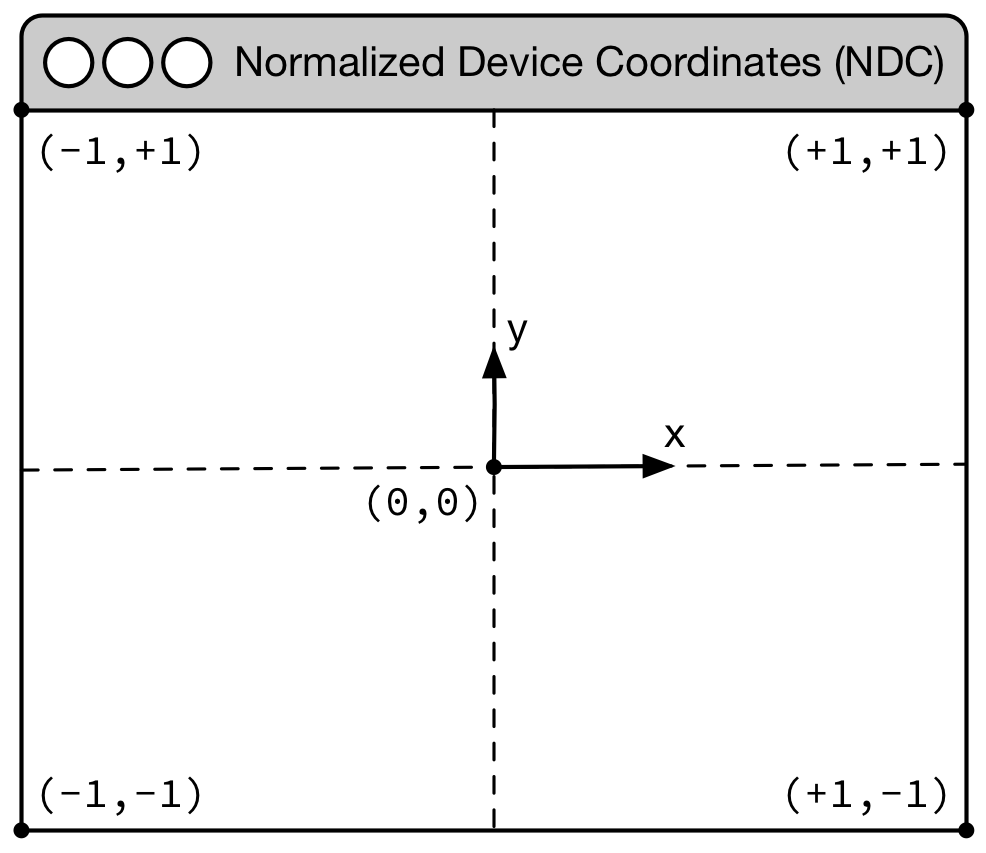
Before even diving into actual code, it is important to understand first how
OpenGL handles coordinates. More precisely, OpenGL considers only coordinates
(x,y,z) that fall into the space where -1 ≤ x,y,z ≤ +1. Any coordinates
that are outside this range will be discarded or clipped (i.e. won't be visible
on screen). This is called Normalized Device Coordinates, or NDC for short.
This is something you cannot change because it is part of the OpenGL API and
implemented in your hardware (GPU). Consequently, even if you intend to render
the whole universe, you'll have utlimately to fit it into this small volume.
The second important fact to know is that x coordinates increase from left to right and y coordinates increase from bottom to top. For this latter one, it is noticeably different from the usual convention and this might induce some problems, especially when you're dealing with the mouse pointer whose y coordinate goes the other way around.
Triangulation
Figure
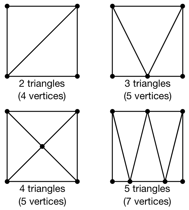
Triangulation of a surface means to find a set of triangles, which covers a given surface. This can be a tedious process but fortunately, there exist many different methods and algorithms to perform such triangulation automatically for any 2D or 3D surface. The quality of the triangulation is measured in terms of the closeness to the approximated surface, the number of triangles necessary (the smaller, the better) and the homogeneity of the triangles (we prefer to have triangles that have more or less the same size and to not have any degenerated triangle).
In our case, we want to render a square and we need to find the proper triangulation (which is not unique as illustrated on the figure). Since we want to minimize the number of triangles, we'll use the 2 triangles solution that requires only 4 (shared) vertices corresponding to the four corners of the quad. However, you can see from the figure that we could have used different triangulations using more vertices, and later in this book we will just do that (but for a reason).
Considering the NDC, our quad will thus be composed of two triangles:
- One triangle described by vertices
(-1,+1), (+1,+1), (-1,-1) - One triangle described by vertices
(+1,+1), (-1,-1), (+1,-1)
Here we can see that vertices (-1,-1) and (+1,+1) are common to both triangles. So instead of using 6 vertices to describe the two triangles, we can
re-use the common vertices to describe the whole quad. Let's name them:
V₀:(-1,+1)V₁:(+1,+1)V₂:(-1,-1)V₃:(+1,-1)
Our quad can now be using triangle (V₀,V₁,V₂) and triangle (V₁,V₂,V₃). This
is exactly what we need to tell OpenGL.
GL Primitives
Figure
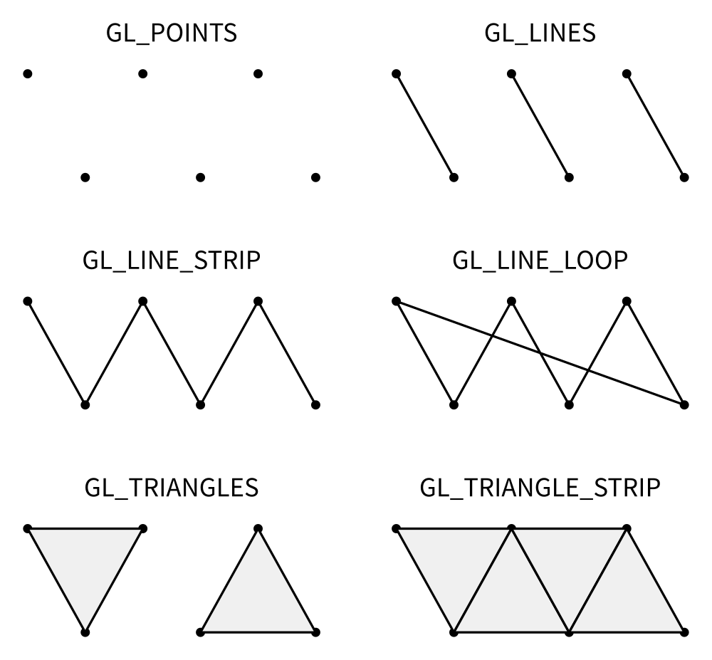
Ok, now things are getting serious because we need to actually tell OpenGL what to do with the vertices, i.e. how to render them? What do they describe in terms of geometrical primitives? This is quite an important topic since this will determine how fragments will actually be generated as illustrated on the image below:
Mostly, OpenGL knows how to draw (ugly) points, (ugly) lines and (ugly)
triangles. For lines and triangles, there exist some variations depending if
you want to specify very precisely what to draw or if you can take advantage of
some implicit assumptions. Let's consider lines first for example. Given a set
of four vertices (V₀,V₁,V₂,V₃), you migh want to draw segments
(V₀,V₁)``(V₂,V₃) using GL_LINES or a broken line (V₀,V₁,V₂,V₃) using
using GL_LINE_STRIP or a closed broken line (V₀,V₁,V₂,V₃,V₀,) using
GL_LINE_LOOP. For triangles, you have the choices of specifying each triangle
individually using GL_TRIANGLES or you can tell OpenGL that triangles follow
an implicit structure using GL_TRIANGLE_STRIP. For example, considering a set
of vertices (Vᵢ), GL_TRIANGLE_STRIP will produce triangles (Vᵢ,Vᵢ₊₁,Vᵢ₊₂).
There exist other primitives but we won't used them in this book because
they're mainly related to geometry shaders that are not introduced.
If you remember the previous section where we explained that our quad can be
described using using triangle (V₀,V₁,V₂) and triangle (V₁,V₂,V₃), you can
now realize that we can take advantage or the GL_TRIANGLE_STRIP primitive
because we took care of describing the two triangles following this implicit
structure.
Interpolation
Figure
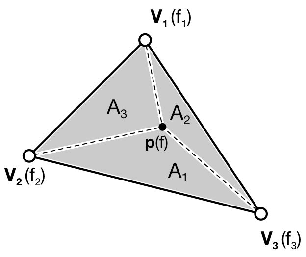
f of a fragment p is given by f = 𝛌₁f₁ +
𝛌₂f₂ + 𝛌₃f₃The choice of the triangle as the only surface primitive is not an arbitrary
choice, because a triangle offers the possibility of having a nice and intuitive
interpolation of any point that is inside the triangle. If you look back at
the graphic pipeline as it has been introduced in the Modern OpenGL section,
you can see that the rasterisation requires for OpenGL to generate fragments
inside the triangle but also to interpolate values (colors on the figure). One
of the legitimate questions to be solved is then: if I have a triangle
(V₁,V₂,V₃), each summit vertex having (for example) a different color, what is
the color of a fragment p inside the triangle? The answer is barycentric
interpolation
as illustrated on the figure on the right.
More precisely, for any point p inside a triangle A = (V₁,V₂,V₃), we consider
triangles:
A₁ = (P,V₂,V₃)A₂ = (P,V₁,V₃)A₃ = (P,V₁,V₂)
And we can define (using area of triangles):
𝛌₁ = A₁/A𝛌₂ = A₂/A𝛌₃ = A₃/A
Now, if we attach a value f₁ to vertex V₁, f₂ to vertex V₂ and f₃ to
vertex V₃, the interpolated value f of p is given by: f = 𝛌₁f₁ + 𝛌₂f₂ +
𝛌₃f₃ You can check by yourself that if the point p is on a border of the
triangle, the resulting interpolated value f is the linear interpolation of
the two vertices defining the segment the point p belongs to.
This barycentric interpolation is important to understand even if it is done automatically by OpenGL (with some variation to take projection into account). We took the example of colors, but the same interpolation scheme holds true for any value you pass from the vertex shader to the fragment shader. And this property will be used and abused in this book.
The hard way
Having reviewed some important OpenGL concepts, it's time to code our quad example. But, before even using OpenGL, we need to open a window with a valid GL context. This can be done using a toolkit such as Gtk, Qt or Wx or any native toolkit (Windows, Linux, OSX). Unfortunately, the Tk Python interface does not allow to create a GL context and we cannot use it. Note there also exists dedicated toolkits such as GLFW or GLUT and the advantage of GLUT is that it's already installed alongside OpenGL. Even if it is now deprecated, we'll use GLUT since it's a very lightweight toolkit and does not require any extra package. Here is a minimal setup that should open a window with a black background.
import sys
import OpenGL.GL as gl
import OpenGL.GLUT as glut

def display():
    gl.glClear(gl.GL_COLOR_BUFFER_BIT)
    glut.glutSwapBuffers()

def reshape(width,height):
    gl.glViewport(0, 0, width, height)

def keyboard( key, x, y ):
    if key == b'\x1b':
        sys.exit( )

glut.glutInit()
glut.glutInitDisplayMode(glut.GLUT_DOUBLE | glut.GLUT_RGBA)
glut.glutCreateWindow('Hello world!')
glut.glutReshapeWindow(512,512)
glut.glutReshapeFunc(reshape)
glut.glutDisplayFunc(display)
glut.glutKeyboardFunc(keyboard)
glut.glutMainLoop()
Note
You won't have access to any GL command before the glutInit() has been
executed because no OpenGL context will be available before this command is
executed.
The glutInitDisplayMode tells OpenGL what are the GL context properties. At
this stage, we only need a swap buffer (we draw on one buffer while the other
is displayed) and we use a full RGBA 32 bits color buffer (8 bits per channel).
The reshape callback informs OpenGL of the new window size while the
display method tells OpenGL what to do when a redraw is needed. In this
simple case, we just ask OpenGL to swap buffers (this avoids flickering).
Finally, the keyboard callback allows us to exit by pressing the Escape key.
Writing shaders
Now that your window has been created, we can start writing our program, that
is, we need to write a vertex and a fragment shader. For the vertex shader, the
code is very simple because we took care of using the normalized device
coordinates to describe our quad in the previous section. This means vertices
do not need to be transformed. Nonetheless, we have to take care of sending 4D
coordinates even though we'll transmit only 2D coordinates (x,y) or the final
result will be undefined. For coordinate z we'll just set it to 0.0 (but
any value would do) and for coordinate w, we set it to 1.0 (see section
Basic Mathematics for the explanation). Note also the (commented)
alternative ways of writing the shader.
attribute vec2 position;
void main()
{
  gl_Position = vec4(position, 0.0, 1.0);

  // or gl_Position.xyzw = vec4(position, 0.0, 1.0);

  // or gl_Position.xy = position;
  //    gl_Position.zw = vec2(0.0, 1.0);

  // or gl_Position.x = position.x;
  //    gl_Position.y = position.y;
  //    gl_Position.z = 0.0;
  //    gl_Position.w = 1.0;
}
For the fragment shader, it is even simpler. We set the color to red which is
described by the tuple (1.0, 0.0, 0.0, 1.0) in normalized RGBA
notation. 1.0 for alpha channel means fully opaque.
void main()
{
  gl_FragColor = vec4(1.0, 0.0, 0.0, 1.0);

  // or gl_FragColor.rgba = vec4(1.0, 0.0, 0.0, 1.0);

  // or gl_FragColor.rgb = vec3(1.0, 0.0, 0.0);
  //    gl_FragColor.a = 1.0;
}
Compiling the program
We wrote our shader and we need now to build a program that will link the vertex and the fragment shader together. Building such program is relatively straightforward (provided we do not check for errors). First we need to request program and shader slots from the GPU:
program  = gl.glCreateProgram()
vertex   = gl.glCreateShader(gl.GL_VERTEX_SHADER)
fragment = gl.glCreateShader(gl.GL_FRAGMENT_SHADER)
We can now ask for the compilation of our shaders into GPU objects and we log for any error from the compiler (e.g. syntax error, undefined variables, etc):
vertex_code = """
  attribute vec2 position;
  void main() { gl_Position = vec4(position, 0.0, 1.0); } """

fragment_code = """
  void main() { gl_FragColor = vec4(1.0, 0.0, 0.0, 1.0); } """

# Set shaders source
gl.glShaderSource(vertex, vertex_code)
gl.glShaderSource(fragment, fragment_code)

# Compile shaders
gl.glCompileShader(vertex)
if not gl.glGetShaderiv(vertex, gl.GL_COMPILE_STATUS):
    error = gl.glGetShaderInfoLog(vertex).decode()
    print(error)
    raise RuntimeError("Vertex shader compilation error")

gl.glCompileShader(fragment)
if not gl.glGetShaderiv(fragment, gl.GL_COMPILE_STATUS):
    error = gl.glGetShaderInfoLog(fragment).decode()
    print(error)
    raise RuntimeError("Fragment shader compilation error")
Then we link our two objects in into a program and again, we check for errors during the process.
gl.glAttachShader(program, vertex)
gl.glAttachShader(program, fragment)
gl.glLinkProgram(program)

if not gl.glGetProgramiv(program, gl.GL_LINK_STATUS):
    print(gl.glGetProgramInfoLog(program))
    raise RuntimeError('Linking error')
and we can get rid of the shaders, they won't be used again (you can think of
them as .o files in C).
gl.glDetachShader(program, vertex)
gl.glDetachShader(program, fragment)
Finally, we make program the default program to be ran. We can do it now because we'll use a single program in this example:
gl.glUseProgram(program)
Uploading data to the GPU
Next, we need to build CPU data and the corresponding GPU buffer that will hold
a copy of the CPU data (GPU cannot access CPU memory). In Python, things are
grealty facilitated by NumPy that allows to have a precise control over number
representations. This is important because GLES 2.0 floats have to be exactly
32 bits long and a regular Python float would not work (they are actually
equivalent to a C double). So let us specify a NumPy array holding 4×2
32-bits float that will correspond to our 4×(x,y) vertices:
# Build data
data = np.zeros((4,2), dtype=np.float32)
We then create a placeholder on the GPU without yet specifying the size:
# Request a buffer slot from GPU
buffer = gl.glGenBuffers(1)

# Make this buffer the default one
gl.glBindBuffer(gl.GL_ARRAY_BUFFER, buffer)
We now need to bind the buffer to the program, that is, for each attribute present in the vertex shader program, we need to tell OpenGL where to find the corresponding data (i.e. GPU buffer) and this requires some computations. More precisely, we need to tell the GPU how to read the buffer in order to bind each value to the relevant attribute. To do this, GPU needs to know what is the stride between 2 consecutive elements and what is the offset to read one attribute:
                 1ˢᵗ vertex  2ⁿᵈ vertex  3ʳᵈ vertex   …
                ┌───────────┬───────────┬───────────┬┄┄
                ┌─────┬─────┬─────┬─────┬─────┬─────┬─┄
                │  X  │  Y  │  X  │  Y  │  X  │  Y  │ …
                └─────┴─────┴─────┴─────┴─────┴─────┴─┄
     offset 0 → │ (x,y)     └───────────┘
                                stride
In our simple quad scenario, this is relatively easy to write because we have a
single attribute ("position"). We first require the attribute location
inside the program and then we bind the buffer with the relevant offset.
stride = data.strides[0]

offset = ctypes.c_void_p(0)
loc = gl.glGetAttribLocation(program, "position")
gl.glEnableVertexAttribArray(loc)
gl.glBindBuffer(gl.GL_ARRAY_BUFFER, buffer)
gl.glVertexAttribPointer(loc, 2, gl.GL_FLOAT, False, stride, offset)
We're basically telling the program how to bind data to the relevant attribute. This is made by providing the stride of the array (how many bytes between each record) and the offset of a given attribute.
Let's now fill our CPU data and upload it to the newly created GPU buffer:
# Assign CPU data
data[...] = (-1,+1), (+1,+1), (-1,-1), (+1,-1)

# Upload CPU data to GPU buffer
gl.glBufferData(gl.GL_ARRAY_BUFFER, data.nbytes, data, gl.GL_DYNAMIC_DRAW)
Rendering
We're done, we can now rewrite the display function:
def display():
    gl.glClear(gl.GL_COLOR_BUFFER_BIT)
    gl.glDrawArrays(gl.GL_TRIANGLE_STRIP, 0, 4)
    glut.glutSwapBuffers()

Figure
The 0,4 arguments in the glDrawArrays tells OpenGL we want to display 4
vertices from our current active buffer and we start at vertex 0. You should
obtain the figure on the right with the same red (boring) color. The whole
source ia available from code/chapter-03/glut-quad-solid.py.
All these operations are necessary for displaying a single colored quad on screen and complexity can escalate pretty badly if you add more objects, projections, lighting, texture, etc. This is the reason why we'll stop using the raw OpenGL interface in favor of a library. We'll use the glumpy library, mostly because I wrote it, but also because it offers a tight integration with numpy. Of course, you can design your own library to ease the writing of GL Python applications.
Uniform color

Figure
uniform variable specifying the color of the
quad.In the previous example, we hard-coded the red color inside the fragment shader
source code. But what if we want to change the color from within the Python
program? We could rebuild the program with the new color but that would not be
very efficient. Fortunately there is a simple solution provided by OpenGL:
uniform. Uniforms, unlike attributes, do not change from one vertex to the
other and this is precisely what we need in our case. We thus need to slightly
modify our fragment shader to use this uniform color:
uniform vec4 color;
void main()
{
  gl_FragColor = color;
}
Of course, we also need to upload a color to this new uniform location and this is easier than for attribute because the memory has already been allocated on the GPU (since the size is know and does not depend on the number of vertices).
loc = gl.glGetUniformLocation(program, "color")
gl.glUniform4f(loc, 0.0, 0.0, 1.0, 1.0)
If you run the new code/glut-quad-uniform-color.py example, you should obtain the blue quad as shown on the right.
Varying color
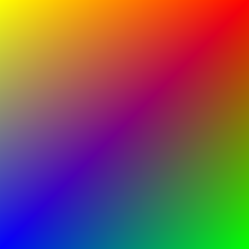
Figure
Until now, we have been using a constant color for the four vertices of our quad and the result is (unsurprisingly) a boring uniform red or blue quad. We can make it a bit more interesting though by assigning different colors to each vertex and see how OpenGL will interpolate colors. Our new vertex shader would need to be rewritten as:
attribute vec2 position;
attribute vec4 color;
varying vec4 v_color;
void main()
{
  gl_Position = vec4(position, 0.0, 1.0);
  v_color= color;
}
We just added our new attribute color but we also added a new variable type:
varying. This type is actually used to transmit a value from the vertex
shader to the fragment shader. As you might have guessed, the varying type
means this value won't be constant over the different fragments but will be
interpolated depending on the relative position of the fragment in the
triangle, as I explained in the Interpolation section. Note that we also
have to rewrite our fragment shader accordingly, but now the v_color will be
an input:
varying vec4 v_color;
void main()
{
  gl_FragColor = v_color;
}
We now need to upload vertex color to the GPU. We could create a new vertex
dedicated buffer and bind it to the new color attribute, but there is a more
interesting solution. We'll use instead a single numpy array and a single buffer,
taking advantage of the NumPy structured array:
data = np.zeros(4, [("position", np.float32, 2),
                    ("color",    np.float32, 4)])
data['position'] = (-1,+1), (+1,+1), (-1,-1), (+1,-1)
data['color']    = (0,1,0,1), (1,1,0,1), (1,0,0,1), (0,0,1,1)
Our CPU data structure is thus:
           1ˢᵗ vertex              2ⁿᵈ vertex
   ┌───────────────────────┬───────────────────────┬┄
   ┌───┬───┬───┬───┬───┬───┬───┬───┬───┬───┬───┬───┬─┄
   │ X │ Y │ R │ G │ B │ A │ X │ Y │ R │ G │ B │ A │ …
   └───┴───┴───┴───┴───┴───┴───┴───┴───┴───┴───┴───┴─┄
   ↑       ↑               └───────────────────────┘
 position  color                     stride
 offset    offset
Binding the buffer is now a bit more complicated but it is made relatively easy thanks to NumPy:
stride = data.strides[0]
offset = ctypes.c_void_p(0)
loc = gl.glGetAttribLocation(program, "position")
gl.glEnableVertexAttribArray(loc)
gl.glBindBuffer(gl.GL_ARRAY_BUFFER, buffer)
gl.glVertexAttribPointer(loc, 2, gl.GL_FLOAT, False, stride, offset)

offset = ctypes.c_void_p(data.dtype["position"].itemsize)
loc = gl.glGetAttribLocation(program, "color")
gl.glEnableVertexAttribArray(loc)
gl.glBindBuffer(gl.GL_ARRAY_BUFFER, buffer)
gl.glVertexAttribPointer(loc, 4, gl.GL_FLOAT, False, stride, offset)
The easy way
As we've seen in the previous section, displaying a simple quad using modern GL is quite tedious and requires a fair number of operations and this is why, from now on, we'll use glumpy whose goal is to make this process both easy and intuitive.
Glumpy is organized around three main modules:
- The Application layer (
app) package is responsible for opening a window and handling user events such as mouse and keyboard interactions. - The OpenGL object oriented layer (
gloo) package is responsible for handling shader programs and syncing CPU/GPU data through the numpy interface. - The Graphic layer (
graphics) package provides higher-level common objects such as text, collections and widgets.
Those modules will help us writing any OpenGL program quite easily. Let's consider again our quad example:
Note
Glumpy will look for any available backend in a given order, starting by GLFW. I strongly advise to install the GLFW package on your system since this backend is activately maintainted and "just works".
We still need to open a window, but now this is straightforward:
from glumpy import app, gloo, gl

# Create a window with a valid GL context
window = app.Window()
If necessary, you can also indicate which backend to use by writing
app.use("glfw") before creating the window. The creation of the program is
also straightforward:
# Build the program and corresponding buffers (with 4 vertices)
quad = gloo.Program(vertex, fragment, count=4)
With the above line, both the CPU data and GPU data (buffer) have been created
and no extra command is necessary at this stage and uploading the data is only
a matter of setting the different fields of the quad program:
# Upload data into GPU
quad['position'] = (-1,+1), (+1,+1), (-1,-1), (+1,-1)
Under the hood, glumpy has parsed your shader programs and has identified
attributes. Rendering is just a matter of calling the draw method from our
shader program, using the proper mode.
# Tell glumpy what needs to be done at each redraw
@window.event
def on_draw(dt):
    window.clear()
    quad.draw(gl.GL_TRIANGLE_STRIP)

# Run the app
app.run()
The whole source is available in code/chapter-03/glumpy-quad-solid.py.
If you run this program using the --debug switch, you should obtain the
following output that shows what is being done in the background. More
specifically, you can check that the program is actually compiled and linked
using the specified shaders and that the buffer is created and bound to the
program.
[i] HiDPI detected, fixing window size
[i] Using GLFW (GL 2.1)
[i] Running at 60 frames/second
GPU: Creating program
GPU: Attaching shaders to program
GPU: Creating shader
GPU: Compiling shader
GPU: Creating shader
GPU: Compiling shader
GPU: Linking program
GPU: Activating program (id=1)
GPU: Activating buffer (id=7)
GPU: Creating buffer (id=7)
GPU: Updating position
GPU: Deactivating buffer (id=7)
GPU: Deactivating program (id=1)
Uniform color
Adding a uniform specified color is only a matter of modifying the
fragment shader as in the previous section and directly assigning the color to
the quad program (see code/chapter-03/glumpy-quad-uniform-color.py):
quad["color"] = 0,0,1,1
Varying color
Adding a per-vertex color is also only a matter of modifying the fragment shader as in the previous section and directly assigning the color to the quad program (see code/chapter-03/glumpy-quad-varying-color.py):
quad["color"] = (1,1,0,1), (1,0,0,1), (0,0,1,1), (0,1,0,1)
Exercises
Now we can play a bit with the shader and hopefully you'll understand why learning to program the dynamic graphic pipeline is worth the effort. Modifying the rendering is now a matter of writing the proper shader. We'll get a first taste in the three exercises below but we'll see much more powerful shader tricks in the next chapters.
Figure
Scaling the quad We've been using previously a uniform to pass a color to
the fragment shader, but we could have used also in the vertex shader to pass
any kind of information. In this exercise, try to modify the vertex shader in
the varying color example in
order for the quad to be animated and to scale with time as shown in the figure
on the right. You will need to update the scale factor within the Python
program, for example in the draw function.
Solution: code/chapter-03/quad-scale.py
Figure
Rotating the quad Let's now rotate the quad as in the figure on the right.
Note that you have access to the cos and sin functions from within the
shader. If you forgot your geometry, here is a quick reminder for a rotation of
angle theta around the origin (0,0) for a point (x,y):
float x2 = cos(theta)*x - sin(theta)*y;
float y2 = sin(theta)*x + cos(theta)*y;
Solution: code/chapter-03/quad-rotation.py
Basic Mathematics
.
There is no way around mathematics. If you want to understand computer geometry, you need to master a few mathematical concepts. But not that many actually. I won't introduce everything since there is already a lot of tutorials online explaining the core concepts of linear algrebra, Euclidean geometry, homogeneous coordinates, projective geometry and quaternions (yes, those are the keywords to enter in your preferred search engine). The teaser image above comes from the Cyclopaedia, an Universal Dictionary of Arts and Sciences published by Ephraim Chambers in London in 1728 (sources History of Geometry).
Projective Geometry
Homogeneous coordinates
Even though we're dealing with the three-dimensional Euclidean space, three
dimensional coordinates are actually not the best representation we can use and
this is the reason why we will use homogeneous coordinates that describe
coordinates in a four-dimensional projective space (that includes the Euclidean
space). We'll see in the next section that this allows us to express linear
transformations (rotation, scaling), affine transformations (translations) and
projection using 4×4 matrices. Homogeneous coordinatess are tightly linked with
regular 3D coordinates with the noticeable difference that they require a
fourth w coordinate that corresponds to the fourth dimension, let's call it
the projective dimension. In order to explain it, we'll use a 1-dimensional
space where point coordinates are single scalars indicating the position of the
points onto the X-axis. This will make everything clearer hopefully.
Let us consider for example a simple set of points [-1.0, -0.5, 0.0, +0.5,
+1.0] in this unidimensional space. We want to project onto another segment
[-2,+2] that represents the screen (any point projected outside this segment
is discared and won't be visible into the final projection). The question now is
how do we project the points onto the screen?
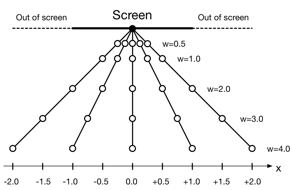
Figure
[-1.0, -0.5, 0.0, +0.5, +1.0].To answer this question, we need to know where is the camera (from where do we
look at the scene) and where are the points positioned relatively to the
screen. This is the reason why we introduce a supplementary w coordinate in
order to indicate the distance to the screen. To go from our Euclidean
representation to our new homogeneous representation, we'll use a conventional
and default value of 1 for all the w such that our new point set is now
[(-1.0,1.0), -(0.5,1.0), (0.0,1.0), (+0.5,1.0), (+1.0,1.0)]. Reciprocally, a
point (x,w) in projective space corresponds to the point x/w (if w ≠ 0)
in our unidimensional Euclidean space. From this conversion, we can see
immediately that there exists actually an infinite set of homogenous coordinates
that correspond to a single Cartesian coordinate as illustrated on the figure.

Figure
Projections
We are now ready to project our point set onto the screen. As shown on the
figure above, we can use an orthographic (all rays are parallel) or a linear
projection (rays originate from the camera point and hit the screen, passing
through points to be projected). For these two projections, results are similar
but different. In the first case, distances have been exactly conserved while
in the second case, the distance between projected points has increased, but
projected points are still equidistant. The third projection is where
homogenous coordinates make sense. For this (arbitrary) projection, we decided
that the further the point is from the origin, the further away from the
origin its projection will be. To do that, we measure the distance of the point
to the origin and we add this distance to its w value before projecting it
(this corresponds to the black circles on the figure) using the linear
projection. It is to be noted that this new projection does not conserve the
distance relationship and if we consider the set of projected points [P(-1.0),
P(-0.5), P(0.0), P(+0.5), P(+1.0)], we have ║P(-1.0)-P(-0.5)]║ >
║P(-0.5)- P(0.0)║.
Note
Quaternions are not homogenous coordinates even though they are usually represented in the form of a 4-tuple (a,b,c,d) that is a shortcut for the actual representation: a + bi⃗ + cj⃗ + dk⃗, where a, b, c, and d are real numbers, and i⃗, j⃗, k⃗ are the fundamental quaternion units.
Back to our regular 3D-Euclidean space, the principle remains the same and we have the following relationship between Cartesian and homogeneous coordinates:
 (x,y,z,w) → (x/w, y/w, z/w) (for w ≠ 0)
Homogeneous    Cartesian

 (x,y,z)   → (x, y, z, 1)
Cartesian     Homogeneous
If you didn't understand everything, you can stick to the description provided by Sam Hocevar:
- If w = 1, then the vector (x,y,z,1) is a position in space
- If w = 0, then the vector (x,y,z,0) is a direction
Transformations
Figure
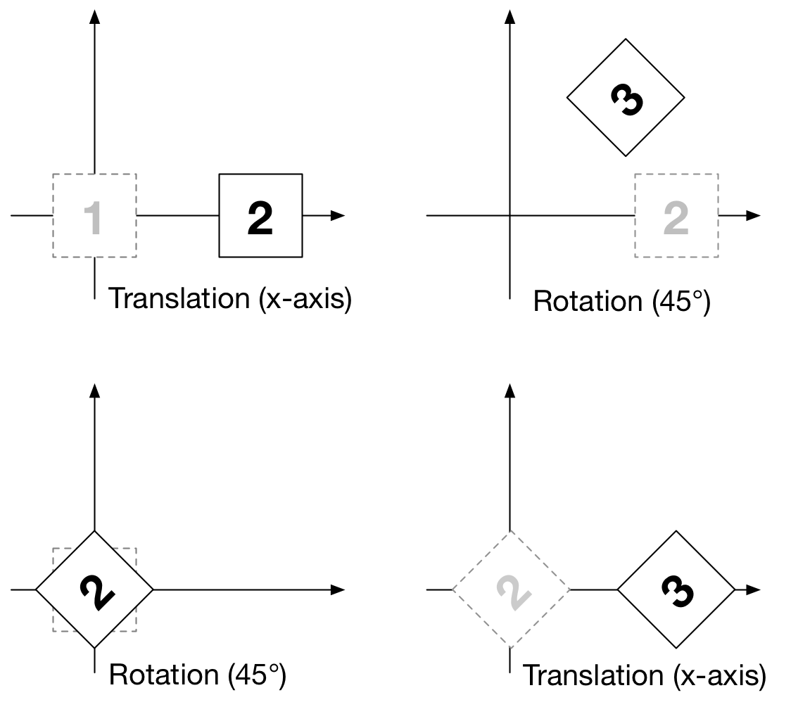
We'll now use homogeneous coordinates and express all our transformations using only 4×4 matrices. This will allow us to chain several transformations by multiplying transformation matrices. However, before diving into the actual definition of these matrices, we need to decide if we consider a four coordinates vector to be 4 rows and 1 column or 1 row and 4 columns. Depending on the answer, the multiplication with a matrix will happen on the left or on the right side of the vector. To be consistent with OpenGL convention, we'll consider a vector to be 4 rows and 1 columns, meaning transformations happen on the left side of vectors. To transform a vertex V by a transformation matrix M, we write: V' = M*V. To chain two transformations M1 and M2 (first M1, then M2), we write: V' = M2*M1*V which is different from V' = M1*M2*V because matrix multiplication is not commutative. As clearly illustrated by the figure on the right, this means for example that a rotation followed by a translation is not the same as a translation followed by a rotation.
Translation
Considering a vertex V = (x, y, z, 1) and a translation vector T = (tx, ty,
tz, 0), the translation of V by T is (x+tx, y+ty, z+tz, 1). The
corresponding matrix is given below:
┌          ┐   ┌   ┐   ┌                        ┐   ┌      ┐
│ 1 0 0 tx │ * │ x │ = │ 1*x + 0*y + 0*z + tx*1 │ = │ x+tx │
│ 0 1 0 ty │   │ y │   │ 0*x + 1*y + 0*z + ty*1 │   │ y+ty │
│ 0 0 1 tz │   │ z │   │ 0*x + 0*y + 1*z + tz*1 │   │ z+tz │
│ 0 0 0 1  │   │ 1 │   │ 0*x + 0*y + 0*z +  1*1 │   │ 1    │
└          ┘   └   ┘   └                        ┘   └      ┘
Scaling
Considering a vertex V = (x, y, z, 1) and a scaling vector S = (sx, sy, sz,
0), the scaling of V by S is (sx*x, sy*y, sz*z, 1). The corresponding
matrix is given below:
┌            ┐   ┌   ┐   ┌                          ┐   ┌      ┐
│ sx 0  0  0 │ * │ x │ = │ sx*x +  0*y +  0*z + 0*1 │ = │ sx*x │
│ 0  sy 0  0 │   │ y │   │  0*x + sy*y +  0*z + 0*1 │   │ sy*y │
│ 0  0  sz 0 │   │ z │   │  0*x +  0*y + sz*z + 0*1 │   │ sz*z │
│ 0  0  0  1 │   │ 1 │   │  0*x +  0*y +  0*z + 1*1 │   │ 1    │
└            ┘   └   ┘   └                          ┘   └      ┘
Rotation
A rotation is defined by an axis of rotation A and an angle of rotation d. We defined below only the most common rotations, that is, around the X-axis, Y-axis and Z-axis.
X-axis rotation
┌                    ┐   ┌   ┐   ┌                                 ┐
│ 1   0       0    0 │ * │ x │ = │ 1*x      + 0*y      + 0*z + 0*1 │
│ 0 cos(d) -sin(d) 0 │   │ y │   │ 0*x + cos(d)*y - sin(d)*z + 0*1 │
│ 0 sin(d)  cos(d) 0 │   │ z │   │ 0*x + sin(d)*y + cos(d)*z + 0*1 │
│ 0   0       0    1 │   │ 1 │   │ 0*x      + 0*y +      0*z + 1*1 │
└                    ┘   └   ┘   └                                 ┘
                                 ┌                      ┐
                               = │ x                    │
                                 │ cos(d)*y - sin(d)*z  │
                                 │ sin(d)*y + cos(d)*z  │
                                 │ 1                    │
                                 └                      ┘
Y-axis rotation
┌                    ┐   ┌   ┐   ┌                                  ┐
│  cos(d) 0 sin(d) 0 │ * │ x │ = │  cos(d)*x + 0*y + sin(d)*z + 0*1 │
│    0    1   0    0 │   │ y │   │       0*x + 1*y +      0*z + 0*1 │
│ -sin(d) 0 cos(d) 0 │   │ z │   │ -sin(d)*x + 0*y + cos(d)*z + 0*1 │
│    0    0    0   1 │   │ 1 │   │       0*x + 0*y      + 0*z + 1*1 │
└                    ┘   └   ┘   └                                  ┘
                                 ┌                      ┐
                               = │ cos(d)*x + sin(d)*z  │
                                 │ y                    │
                                 │ -sin(d)*x + cos(d)*z │
                                 │ 1                    │
                                 └                      ┘
Z-axis rotation
┌                    ┐   ┌   ┐   ┌                                  ┐
│ cos(d) -sin(d) 0 0 │ * │ x │ = │  cos(d)*x - sin(d)*y + 0*z + 0*1 │
│ sin(d)  cos(d) 0 0 │   │ y │   │  sin(d)*x + cos(d)*y + 0*z + 0*1 │
│   0       0    1 0 │   │ z │   │       0*x +      0*y + 1*z + 0*1 │
│   0       0    0 1 │   │ 1 │   │       0*x +      0*y + 0*z + 1*1 │
└                    ┘   └   ┘   └                                  ┘
                                 ┌                      ┐
                               = │ cos(d)*x - sin(d)*y  │
                                 │ sin(d)*x + cos(d)*y  │
                                 │ z                    │
                                 │ 1                    │
                                 └                      ┘
A word of caution
OpenGL uses a column-major representation of matrices. This mean that when reading a set of 16 contiguous values in memory, relative to a 4×4 matrix, the first 4 values correspond to the first column while in Numpy (using C default layout), this would correspond to the first row. In order to stay consistent with most OpenGL tutorials, we'll use a column-major order in the rest of this book. This means that any glumpy transformations will appear to be transposed when displayed, but the underlying memory representation will still be consistent with OpenGL and GLSL. This is all you need to know at this stage.
Considering a set of 16 contiguous values in memory:
┌                                  ┐
│ a b c d e f g h i j k l  m n o p │
└                                  ┘
We get different representations depending on the order convention (column major or row major):
column-major                          row-major
  (OpenGL)                             (NumPy)
 ┌         ┐   ┌   ┐   ┌         ┐   ┌         ┐   ┌                   ┐
 │ a e i m │ × │ x │ = │ x y z w │ × │ a b c d │ = │ ax + ey + iz + mw │
 │ b f j n │   │ y │   └         ┘   │ e f g h │   │ bx + fy + jz + nw │
 │ c g k o │   │ z │                 │ i j k l │   │ cx + gy + kz + ow │
 │ d h l p │   │ w │                 │ m n o p │   │ dx + hy + lz + pw │
 └         ┘   └   ┘                 └         ┘   └                   ┘
For example, here is a translation matrix as returned by the
glumpy.glm.translation function:
import glumpy
T = glumpy.glm.translation(1,2,3)
print(T)
[[ 1.  0.  0.  0.]
 [ 0.  1.  0.  0.]
 [ 0.  0.  1.  0.]
 [ 1.  2.  3.  1.]]
print(T.ravel())
[ 1.  0.  0.  0.  0.  1.  0.  0.  0.  0.  1.  0.  1.  2.  3.  1.]
                                                  ↑   ↑   ↑
                                                  13  14  15
So this means you would use this translation on the left when uploaded to the GPU, but you would use on the right with Python/NumPy:
T = glumpy.glm.translation(1,2,3)
V = [3,2,1,1]
print(np.dot(V, T))
[ 4.  4.  4.  1.]
Projections
In order to define a projection, we need to specify first what do we want to view, that is, we need to define a viewing volume such that any object within the volume (even partially) will be rendered while objects outside won't. On the image below, the yellow and red spheres are within the volume while the green one is not and does not appear on the projection.
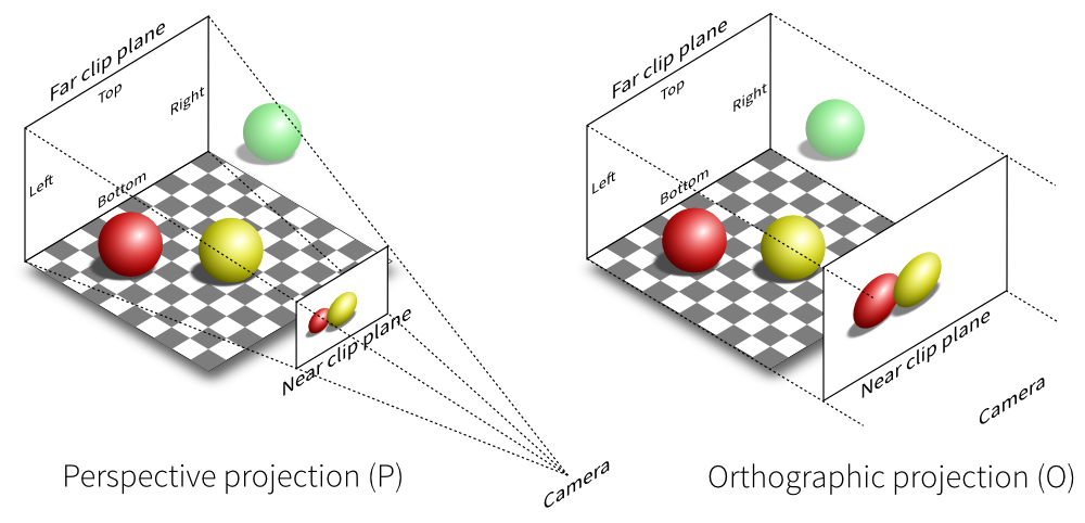
There exist many different ways to project a 3D volume onto a 2D screen but we'll only use the perspective projection (distant objects appear smaller) and the orthographic projection which is a parallel projection (distant objects have the same size as closer ones) as illustrated on the image above. Until now (previous section), we have been using implicitly an orthographic projection in the z=0 plane.
Depending on the projection we want, we will use one of the two projection matrices below:
Orthographic
┌                                         ┐ n: near
│ 2/(r-l)    0       0     -((r+l)/(r-l)) │ f: far
│   0     2/(t-b)    0     -((t+b)/(t-b)) │ t: top
│   0        0    -2/(f-n) -((f+n)/(f-n)) │ b: bottom
│   0        0      -1            0       │ l: left
└                                         ┘ r: right
          Orthographic projection
Perspective
┌                                               ┐ n: near
│ 2n/(r-l)    0       (r+l)/(r-l)       0       │ f: far
│    0     2n/(t-b)   (t+b)/(t-b)       0       │ t: top
│    0        0     -((f+n)/(f-n)) -(2nf/(f-n)) │ b: bottom
│    0        0           -1            0       │ l: left
└                                               ┘ r: right
            Perspective projection
At this point, it is not necessary to understand how these matrices were built. Suffice it to say they are standard matrices in the 3D world. Both assume the viewer (=camera) is located at position (0,0,0) and is looking in the direction (0,0,1).
There exists a second form of the perpective matrix that might be easier to manipulate. Instead of specifying the right/left/top/bottom planes, we'll use field of view in the horizontal and vertical direction:
┌                                     ┐ n: near
│ c/aspect  0       0          0      │ f: far
│    0      c       0          0      │ c: cotangent(fovy)
│    0      0  (f+n)/(n-f)  2nf/(n-f) │
│    0      0      -1          0      │
└                                     ┘
            Perspective projection
where fovy specifies the field of view angle in the y direction
and aspect specifies the aspect ratio that determines the field of view in
the x direction.
Model and view matrices
We are almost done with matrices. You may have guessed that the above matrices require the viewing volume to be in the z direction. We could design our 3D scene such that all objects are within this direction but it would not be very convenient. So instead, we use a view matrix that maps the world space to camera space. This is pretty much as if we were orienting the camera at a given position and look toward a given direction. In the meantime, we can further refine the whole pipeline by providing a model matrix that maps the object's local coordinate space into world space. For example, this is useful for rotating an object around its center. To sum up, we need:
- Model matrix maps from an object's local coordinate space into world space
- View matrix maps from world space to camera space
- Projection matrix maps from camera to screen space
This corresponds to the model-view-projection model. If you have read the whole chapter carefully, you may have guessed the corresponding GLSL shader:
uniform mat4 view;
uniform mat4 model;
uniform mat4 projection;
attribute vec3 P;
void main(void)
{
    gl_Position = projection*view*model*vec4(P, 1.0);
}
Rendering a cube
.
We now have all the pieces needed to render a simple 3D scene, that is, a rotating cube as shown in the teaser image above. But we first need to create the cube and to tell OpenGL how we want to actually project it on the screen.
Object creation
We need to define what we mean by a cube since there is not such thing as as cube in OpenGL. A cube, when seen from the outside has 6 faces, each being a square. We just saw that to render a square, we need two triangles. So, 6 faces, each of them being made of 2 triangles, we need 12 triangles.
How many vertices? 12 triangles × 3 vertices per triangles = 36 vertices might be a reasonable answer. However, we can also notice that each vertex is part of 3 different faces actually. We'll thus use no more than 8 vertices and tell explicitly OpenGL how to draw 6 faces with them:
V = np.zeros(8, [("position", np.float32, 3)])
V["position"] = [[ 1, 1, 1], [-1, 1, 1], [-1,-1, 1], [ 1,-1, 1],
                 [ 1,-1,-1], [ 1, 1,-1], [-1, 1,-1], [-1,-1,-1]]
These vertices describe a cube centered on (0,0,0) that goes from (-1,-1,-1) to
(+1,+1,+1). Unfortunately, we cannot use gl.GL_TRIANGLE_STRIP as we did for
the quad. If you remember how this rendering primitive considers vertices as a
succession of triangles, you should also realize there is no way to organize
our vertices into a triangle strip that would describe our cube. This means we
have to tell OpenGL explicitly what are our triangles, i.e. we need to
describe triangles in terms of vertex indices (relatively to the V array we
just defined):
I = np.array([0,1,2, 0,2,3,  0,3,4, 0,4,5,  0,5,6, 0,6,1,
              1,6,7, 1,7,2,  7,4,3, 7,3,2,  4,7,6, 4,6,5], dtype=np.uint32)
This I is an IndexBuffer that needs to be uploaded to the GPU as well.
Using glumpy, the easiest way is to use a VertexBuffer for vertex data and
an IndexBuffer for index data:
V = V.view(gloo.VertexBuffer)
I = I.view(gloo.IndexBuffer)
We can now proceed with the actual creation of the cube and upload the
vertices. Note that we do not specify the count argument because we'll bind
explicitely our own vertex buffer. The vertex and fragment shader sources
are given below.
cube = gloo.Program(vertex, fragment)
cube["position"] = V
And we'll use the indices buffer when actually rendering the cube.
Scene setup
The next step is to define the scene. This means we need to say where are our objects located and oriented in space, where is our camera located, what kind of camera we want to use and ultimately, where do we look at. In this simple example, we'll use the model-view-projection model that requires 3 matrices:
model:maps from an object's local coordinate space into world spaceview:maps from world space to camera spaceprojection:maps from camera to screen space
The corresponding vertex shader code is then:
vertex = """
uniform mat4   model;
uniform mat4   view;
uniform mat4   projection;
attribute vec3 position;
void main()
{
    gl_Position = projection * view * model * vec4(position,1.0);
} """
and we'll keep the fragment shader to a minimum for now (red color):
fragment = """
void main()
{
    gl_FragColor = vec4(1.0, 0.0, 0.0, 1.0);
} """
For the projection, we'll use the default perspective camera that is available
from the glumpy.glm module (that also defines ortho, frustum and perspective
matrices as well as rotation, translation and scaling operations). This default
perspective matrix is located at the origin and looks in the negative z
direction with the up direction pointing toward the positive y-axis. If we
leave our cube at the origin, the camera would be inside the cube and we would
not see much. So let's first create a view matrix that is a translation along the
z-axis:
view = np.eye(4,dtype=np.float32)
glm.translate(view, 0,0,-5)
Next, we need to define the model matrix and the projection matrix. However,
we'll not setup them right away because the model matrix will be updated in the
on_draw function in order to rotate the cube, while the projection matrix
will be updated as soon as the viewport changes (which is the case when the
window is first created) in the on_resize function.
projection = np.eye(4,dtype=np.float32)
model = np.eye(4,dtype=np.float32)

cube['model'] = model
cube['view'] = view
cube['projection'] = projection
In the resize function, we update the projection with a perspective matrix,
taking the window aspect ratio into account. We define the viewing volume
with near=2.0, far=100.0 and field of view of 45°:
@window.event
def on_resize(width, height):
   ratio = width / float(height)
   cube['projection'] = glm.perspective(45.0, ratio, 2.0, 100.0)
For the model matrix, we want the cube to rotate around its center. We do that
by compositing a rotation about the z axis (theta), then about the y axis (phi):
phi, theta = 0,0

@window.event
def on_draw(dt):
    global phi, theta
    window.clear()
    cube.draw(gl.GL_TRIANGLES, I)

    # Make cube rotate
    theta += 1.0 # degrees
    phi += 1.0 # degrees
    model = np.eye(4, dtype=np.float32)
    glm.rotate(model, theta, 0, 0, 1)
    glm.rotate(model, phi, 0, 1, 0)
    cube['model'] = model
Actual rendering
Figure
We're now alsmost ready to render the whole scene but we need to modify the initialization a little bit to enable depth testing:
@window.event
def on_init():
    gl.glEnable(gl.GL_DEPTH_TEST)
This is needed because we're now dealing with 3D, meaning some rendered triangles may be behind some others. OpenGL will take care of that provided we declared our context with a depth buffer which is the default in glumpy.
As previously, we'll run the program for exactly 360 frames in order to make an endless animation:
app.run(framerate=60, framecount=360)
Complete source code: code/chapter-05/solid-cube.py
Variations
Colored cube
The previous cube is not very interesting because we used a single color for all the faces and this tends to hide the 3D structure. We can fix this by adding some colors and in the process, we'll discover why glumpy is so useful. To add color per vertex to the cube, we simply define the vertex structure as:
V = np.zeros(8, [("position", np.float32, 3),
                 ("color",    np.float32, 4)])
V["position"] = [[ 1, 1, 1], [-1, 1, 1], [-1,-1, 1], [ 1,-1, 1],
                 [ 1,-1,-1], [ 1, 1,-1], [-1, 1,-1], [-1,-1,-1]]
V["color"]    = [[0, 1, 1, 1], [0, 0, 1, 1], [0, 0, 0, 1], [0, 1, 0, 1],
                 [1, 1, 0, 1], [1, 1, 1, 1], [1, 0, 1, 1], [1, 0, 0, 1]]
And we're done ! Well, actually, we also need to slightly modify the vertex shader since color is now an attribute that needs to be passed to the fragment shader.
vertex = """
uniform mat4   model;         // Model matrix
uniform mat4   view;          // View matrix
uniform mat4   projection;    // Projection matrix
attribute vec4 color;         // Vertex color
attribute vec3 position;      // Vertex position
varying vec4   v_color;       // Interpolated fragment color (out)
void main()
{
    v_color = color;
    gl_Position = projection * view * model * vec4(position,1.0);
} """

fragment = """
varying vec4 v_color;         // Interpolated fragment color (in)
void main()
{
    gl_FragColor = v_color;
} """
Figure
Furthermore, since our vertex buffer fields corresponds exactly to program attributes, we can directly bind it:
cube = gloo.Program(vertex, fragment)
cube.bind(V)
But we could also have written
cube = gloo.Program(vertex, fragment)
cube["position"] = V["position"]
cube["color"] = V["color"]
Complete source code: code/chapter-05/color-cube.py
Outlined cube
Figure
GL_POLYGON_OFFSET_FILL that allows to draw
coincident surfaces properly.We can make the cube a bit nicer by outlining it using black lines. To outline the cube, we need to draw lines between pairs of vertices on each face. 4 lines for the back and front face and 2 lines for the top and bottom faces. Why only 2 lines for top and bottom? Because lines are shared between the faces. So overall we need 12 lines and we need to compute the corresponding indices (I did it for you):
O = [0,1, 1,2, 2,3, 3,0,
     4,7, 7,6, 6,5, 5,4,
     0,5, 1,6, 2,7, 3,4 ]
O = O.view(gloo.IndexBuffer)
We then need to draw the cube twice. One time using triangles and the indices index buffer and one time using lines with the outline index buffer. We need also to add some OpenGL black magic to make things nice. It's not very important to understand it at this point but roughly the idea to make sure lines are drawn "above" the cube because we paint a line on a surface:
@window.event
def on_draw(dt):
    global phi, theta, duration

    window.clear()

    # Filled cube
    gl.glDisable(gl.GL_BLEND)
    gl.glEnable(gl.GL_DEPTH_TEST)
    gl.glEnable(gl.GL_POLYGON_OFFSET_FILL)
    cube['ucolor'] = .75, .75, .75, 1
    cube.draw(gl.GL_TRIANGLES, I)

    # Outlined cube
    gl.glDisable(gl.GL_POLYGON_OFFSET_FILL)
    gl.glEnable(gl.GL_BLEND)
    gl.glDepthMask(gl.GL_FALSE)
    cube['ucolor'] = 0, 0, 0, 1
    cube.draw(gl.GL_LINES, O)
    gl.glDepthMask(gl.GL_TRUE)

    # Rotate cube
    theta += 1.0 # degrees
    phi += 1.0 # degrees
    model = np.eye(4, dtype=np.float32)
    glm.rotate(model, theta, 0, 0, 1)
    glm.rotate(model, phi, 0, 1, 0)
    cube['model'] = model
Complete source code: code/chapter-05/outlined-cube.py
Textured cube
Figure
For making a textured cube, we need a texture (a.k.a. an image) and some coordinates to tell OpenGL how to map it to the cube faces. Texture coordinates are normalized and should be inside the [0,1] range (actually, texture coordinates can be pretty much anything but for the sake of simplicity, we'll stick to the [0,1] range). Since we are displaying a cube, we'll use one texture per side and the texture coordinates are quite easy to define: [0,0], [0,1], [1,0] and [1,1]. Of course, we have to take care of assigning the right texture coordinates to the right vertex or you texture will be messed up.
Furthemore, we'll need some extra work because we cannot share anymore our vertices between faces since they won't share their texture coordinates. We thus need to have a set of 24 vertices (6 faces × 4 vertices). We'll use the dedicated function below that will take care of generating the right texture coordinates.
def cube():
    vtype = [('position', np.float32, 3),
             ('texcoord', np.float32, 2)]
    itype = np.uint32

    # Vertices positions
    p = np.array([[1, 1, 1], [-1, 1, 1], [-1, -1, 1], [1, -1, 1],
                  [1, -1, -1], [1, 1, -1], [-1, 1, -1], [-1, -1, -1]],
                  dtype=float)

    # Texture coords
    t = np.array([[0, 0], [0, 1], [1, 1], [1, 0]])

    faces_p = [0, 1, 2, 3,  0, 3, 4, 5,   0, 5, 6, 1,
               1, 6, 7, 2,  7, 4, 3, 2,   4, 7, 6, 5]
    faces_t = [0, 1, 2, 3,  0, 1, 2, 3,   0, 1, 2, 3,
               3, 2, 1, 0,  0, 1, 2, 3,   0, 1, 2, 3]

    vertices = np.zeros(24, vtype)
    vertices['position'] = p[faces_p]
    vertices['texcoord'] = t[faces_t]

    filled = np.resize(
       np.array([0, 1, 2, 0, 2, 3], dtype=itype), 6 * (2 * 3))
    filled += np.repeat(4 * np.arange(6, dtype=itype), 6)

    vertices = vertices.view(gloo.VertexBuffer)
    filled   = filled.view(gloo.IndexBuffer)

    return vertices, filled
Now, inside the fragment shader, we have access to the texture:
vertex = """
uniform mat4   model;      // Model matrix
uniform mat4   view;       // View matrix
uniform mat4   projection; // Projection matrix
attribute vec3 position;   // Vertex position
attribute vec2 texcoord;   // Vertex texture coordinates
varying vec2   v_texcoord;   // Interpolated fragment texture coordinates (out)

void main()
{
    // Assign varying variables
    v_texcoord  = texcoord;

    // Final position
    gl_Position = projection * view * model * vec4(position,1.0);
} """


fragment = """
uniform sampler2D texture; // Texture
varying vec2 v_texcoord;   // Interpolated fragment texture coordinates (in)
void main()
{
    // Get texture color
    gl_FragColor = texture2D(texture, v_texcoord);
} """
Complete source code: code/chapter-05/textured-cube.py
Exercises
Figure
Shader outline We've seen in the section outlined cube how to draw a thin line around the cube to enhance its shape. For this, we drew the cube twice, one for the cube itself and a second time for the outline. However, it is possible to get more or less the same results from within the shader in a single pass. The trick is to pass the (untransformed) position from the vertex shader to the fragment shader and to use this information to set the color of the fragment to either the black color or the v_color. Starting from the color cube code, try to modify only the shader code (both vertex and fragment) to achieve the result on the right.
Solution: code/chapter-05/border-cube.py
Figure
Hollow cube We can play a bit more with the shader and try to draw only a
thick border surrounded by black outline. For the "transparent" part, you'll
need to use the discard instruction from within the fragment shader that
instructs OpenGL to not display the fragment at all and to terminate the
program from this shader. Since nothing will be rendered, there is no need to
process the rest of program.
Solution: code/chapter-05/hollow-cube.py
Anti-grain geometry
.
The late Maxim Shemanarev (1966-2013) designed the anti-grain library, a (very) high quality rendering engine written in C++. The library is both nicely written (one of the best C++ library I've seen with the Eigen library) and heavily documented, but the strongest feature is the quality of the rendering output that is probably one of the best, even 10 years after the library has been released (have look at the demos). This is the level of quality we target in this book. However, OpenGL anti-aliasing techniques (even latest ones) won't do the job and we'll need to take care of pretty much everything.
Antialiasing
Figure
Aliasing is a well known problem in signal processing where it can occur in time (temporal aliasing) or in space (spatial aliasing). In computer graphics, we're mostly interested in spatial aliasing (such a Moiré pattern or jaggies) and the way to attenuate it. Let's first examine the origin of the problem from a practical point of view (have a look at wikipedia for the background theory).
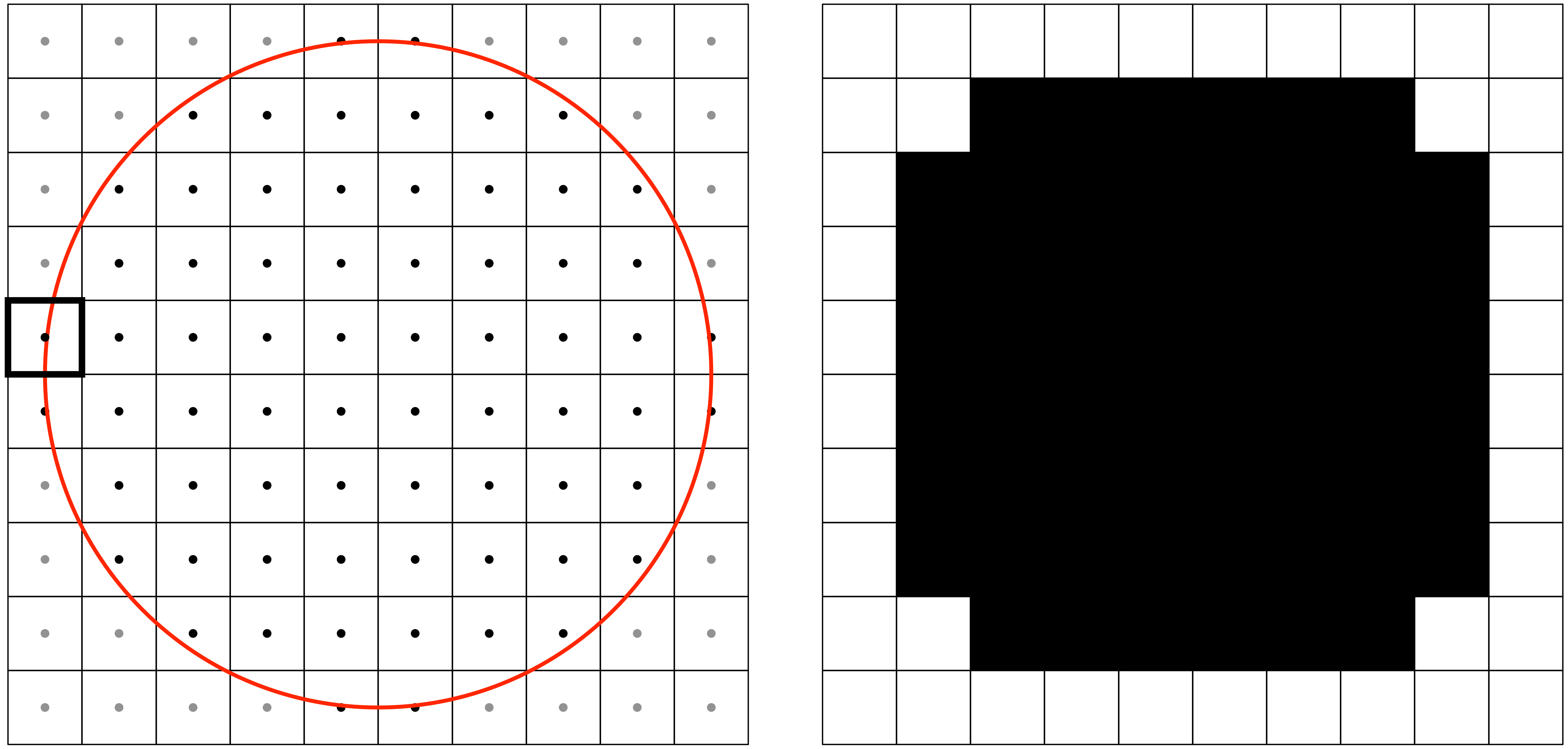
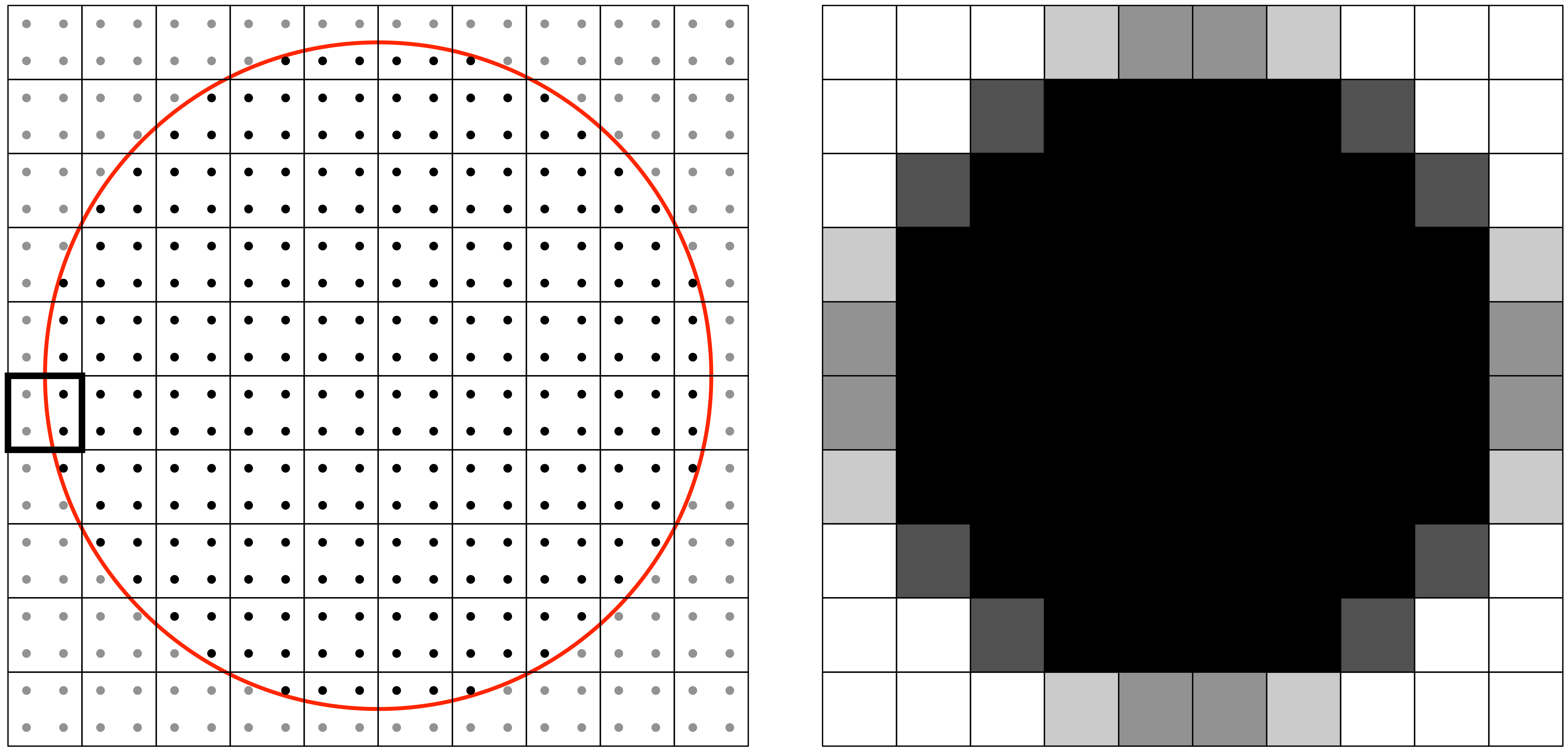
The figure on the right illustrates the problem when we want to render a disc
onto a small area. The very first thing to be noticed is that pixels are
not mathematical points and the center of the pixel is usually associated
with the center of the pixel. This means that if we consider a pair of integer
coordinates (i,j), then (i+Δx, j+Δy) designates the same pixel (with -0.5
< Δx, Δy < 0.5). In order to rasterize the mathematical description of our
circle (center and radius), the rasterizer examines the center of each pixel to
determine if it falls inside or outside the shape. The result is illustrated on
the right part of the figure. Even if the center of a pixel is very close but
outside of the circle, it is not painted as it is shown for the thicker square
on the figure. More generally, without anti-aliasing, a pixel will be only on
(inside) or off (outside), leading to very hard jagged edges and a very
approximate shape for small sizes as well.
Sample based methods
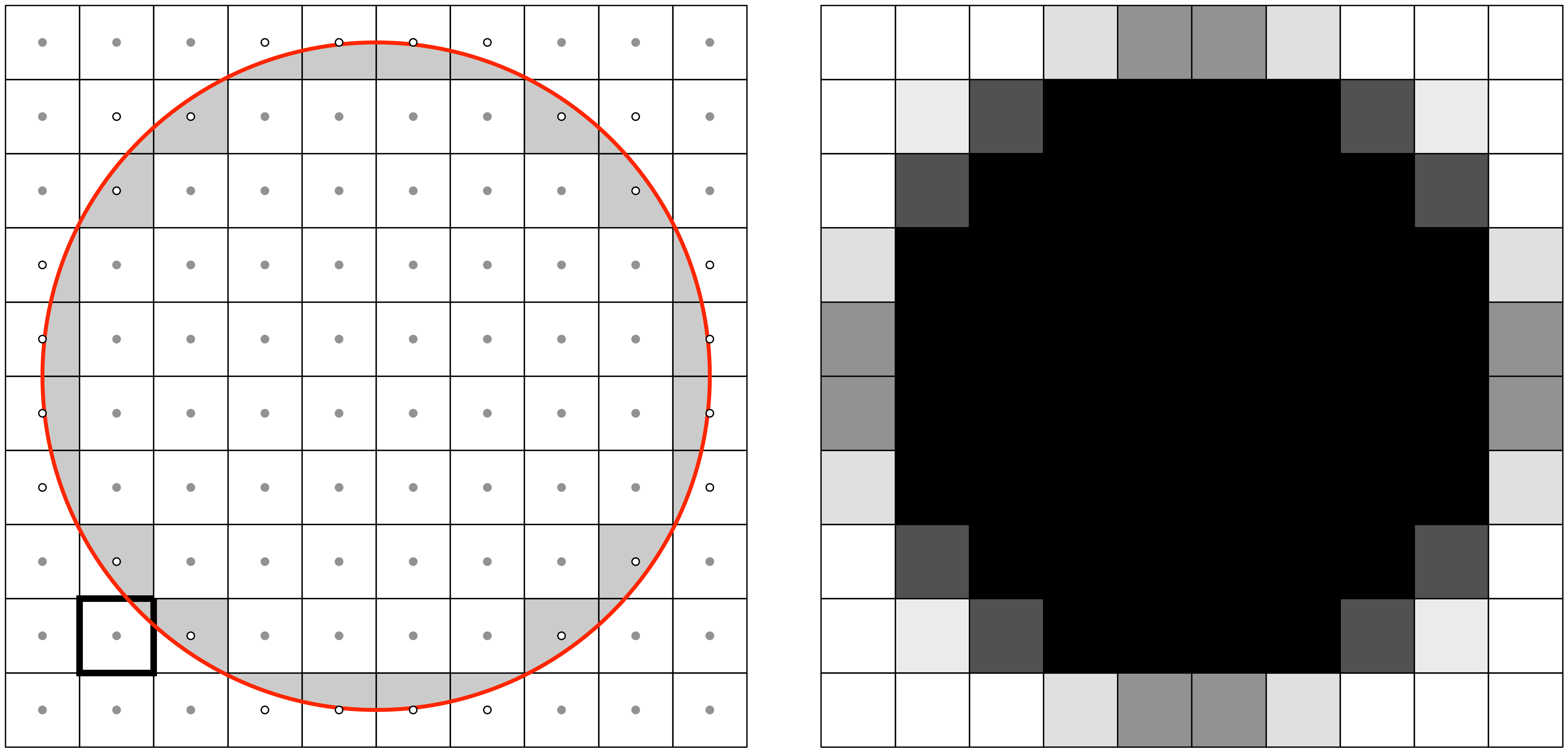
Figure
One of the simplest method to remove antialising consists in using several samples to estimate the final color of a fragment. Instead of only considering the center of the pixel, one case use several samples over the whole surface of a pixel in order to have a better estimate as shown on the figure on the right. A fragment that was previously considered outside, based on its center only, can now be considered half inside / half outside. This multi-sampling helps to attenuate the jagged edges we've seen in the previous section. On the figure, we used a very simple and straightforward multi-sample method, assigning fixed and equidistant locations for the four subsamples. There exist however better methods for multi-sampling as shown by the impressive list of sample based antialiasing techniques:
- SSAA: Supersampling antialiasing
- MSAA: Multisample antialiasing
- FSAA: Full screen anti-aliasing
- FXAA: Fast approximate antialiasing
- SMAA: Subpixel morphological antialiasing
- DLAA: Directionally localized antialiasing
- NFAA: Normal filter antialiasing
- HRAA: High-Resolution antialiasing
- TXAA: Temporal antialiasing
- EQAA: Enhanced quality at-prntialiasing
- CSAA: Coverage Sample antialiasing
Depending on the performance you need to achieve (in terms of rendering quality and speed) one method might be better than the other. However, you cannot expect to achieve top quality due to inherent limitations of all these methods. If they are great for real-time rendering such as video games (and some of them are really good), they are hardly sufficient for any scientific visualization as illustrated on the figure below.
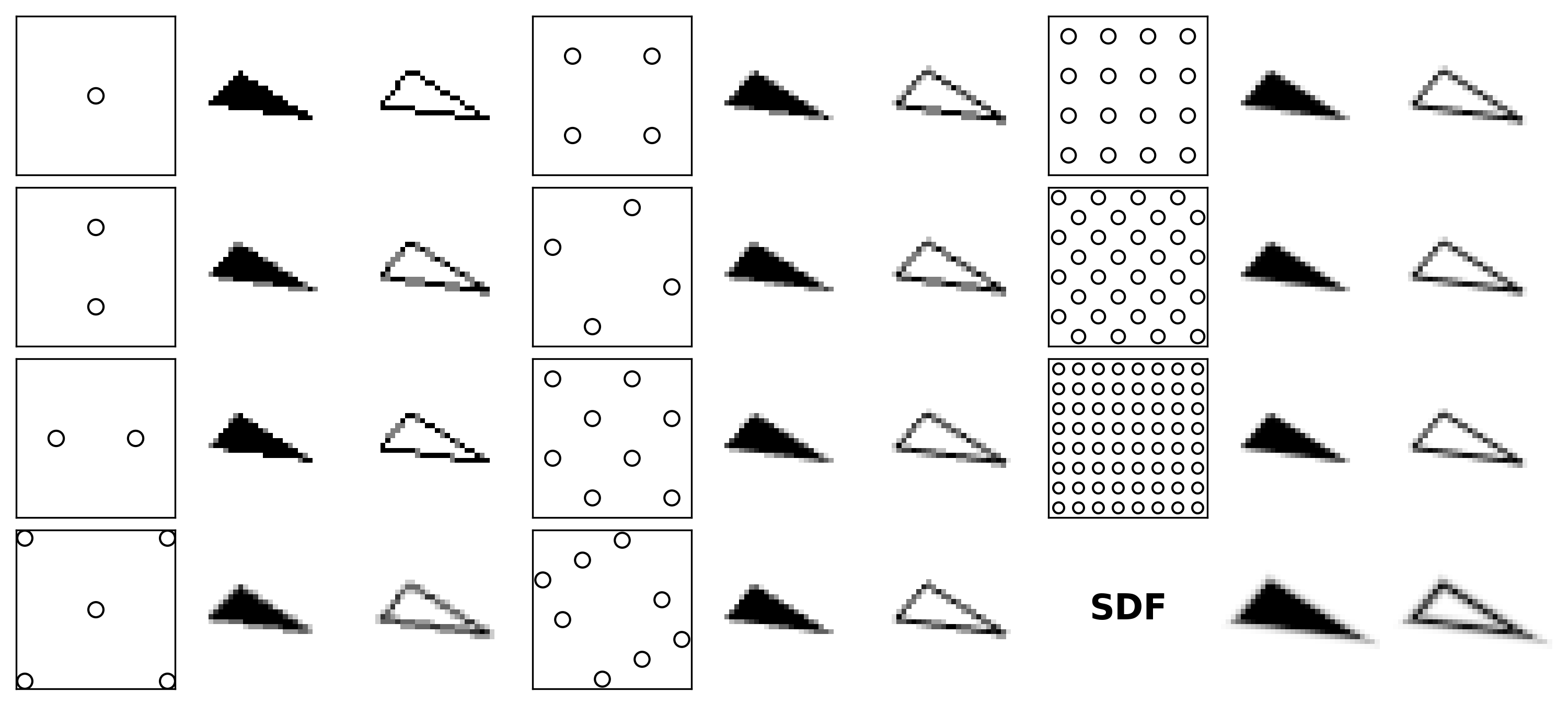
Figure
This is the reason why we won't use them in the rest of this book. If you want more details on these techniques, you can have a look at this reddit discussion explaining antialiasing modes or this nice overview of MSAA
Coverage methods
Figure
Another approach for anti-aliasing is to compute the exact coverage of a shape over each pixel surface as shown on the figure on the right. To do so, we need of course to know precisely the shape we want to display and where it is located in order to compute the coverage of the shape onto the pixel grid. On the image, this corresponds to the grey areas that give us direct access to the final color of the pixel (more precisely, the percentage of the color we have to mix with the background color or any other object in the vicinity). Unfortunately, such method is not possible to enforce in a full 3D scene because all the transformations and differen occlusuins would make the computation of the final shape too complex. In two dimensions however, this is probably the best method we can use and this is also the method that is used in the Anti-grain geometry library that constitutes the quality standard we aim at.
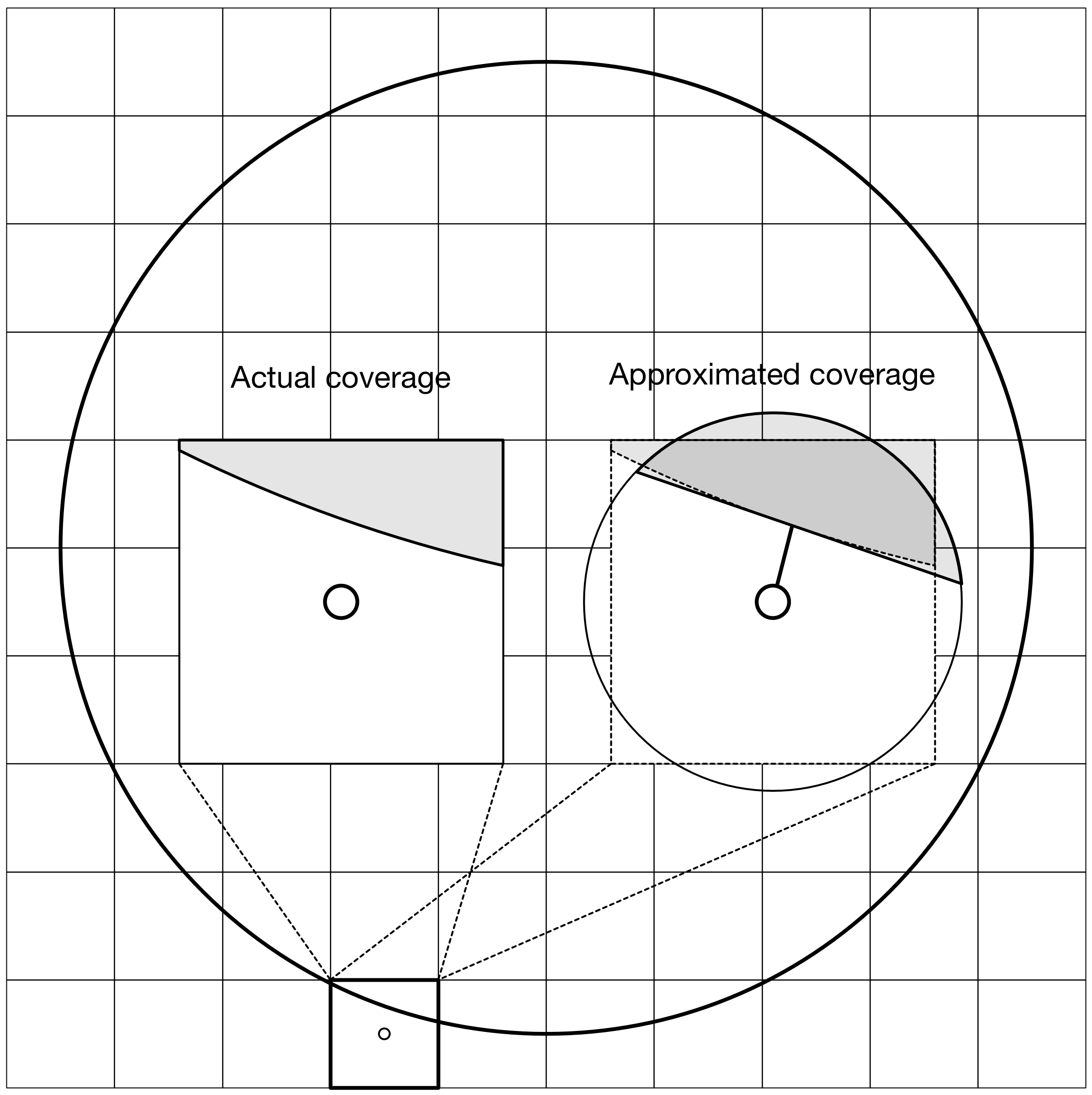
Figure
But even in 2D, computing the exact coverage of the shape over the different pixels can become rapidly a complex and slow task. One way to greatly simplify the problem is to consider pixel to be round (instead of square or rectangle). With such asumption, we only need to compute the distance from the center of the pixel to the border of the shape (that is locally considered to be a line) to get a very accurate estimate of the coverage and this is exactly what we'll do in the next section.
If you wonder if our round pixel shape approximation makes any. sense at all, have a look at the subpixel zoo maintained by Ian Mallett and you'll understand our assumption is not so bad overall.
Signed distance fields
Here comes the fun. After having reviewed different method for anti-aliasing, we (mostly me actually) retained the coverage method that necessitates to evaluate the distance from the center of a pixel to the border of the shape. To do that, we'll use signed distance functions.
Signed distance function
From wikipedia (again):
A signed distance function (or oriented distance function) of a set Ω in a metric space determines the distance of a given point x from the boundary of Ω, with the sign determined by whether x is in Ω. The function has positive values at points x inside Ω, it decreases in value as x approaches the boundary of Ω where the signed distance function is zero, and it takes negative values outside of Ω.
Said differently: in order to render a shape, we need to find a function of
x and y that returns a value that is the signed distance to the shape, that
is, a signed distance to the border of the shape. Inside the shape, the value
is positive, outside the shape the value is negative and on the border, the
value is zero. Easy enough.
Note
The sign of inside/outside can be reversed as long as they are opposite.
Of course, the question is now how do we find such function? Let's start with
the most simple geometrical primitive: a circle centered on (xc,yc) with a
radius r. For any point (x,y), we know the (non-negative) distance to
the center is given by: d = sqrt((x-xc)*(x-xc)+(y-yc)*(y-yc)). To simplify
computations, we'll consider the circle to centered on the origin, the distance
now writes d = sqrt(x*x+y*y). This distance is not what we want since we
target a signed distance to the border of the circle. However, this can be
obtained very easily by subtracting the radius r from d(x,y). In the end,
signed distance from a point (x,y) to a circle of radius r centered on the
origin is given by:
d(x,y) = sqrt(x*x+y*y) - r
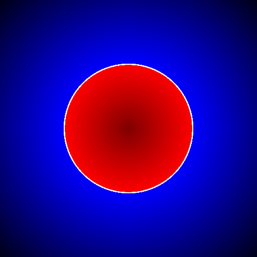
Figure
Signed distance to a circle. Inside is red, outside is blue, border is white.
As an exercise, you can check that d(x,y) is zero if (x,y) is on the
border, strictly negative if (x,y) is inside the circle and strictly positive
outside the circle.
Now, let's check if OpenGL is consistent with our maths. We'll write a fragment shader that compute the color according to the distance to the shape. We'll use the blue color outside the circle, red color inside and white color on the border (with some tolerance or we won't see anything).
float distance(vec2 P, vec2 center, float radius)
{
    return length(P-center) - radius;
}

varying vec2 v_position;
void main()
{
    const float epsilon = 0.005;
    float d = distance(v_position, vec2(0.0), 0.5);
    if (d > +epsilon)
        gl_FragColor = vec4(abs(d), 0.0, 0.0, 1.0);
    else if (d < -epsilon)
        gl_FragColor = vec4(0.0, 0.0, abs(d), 1.0);
    else
        gl_FragColor = vec4(0.0, 0.0, 0.0, 1.0);
}
Geometrical primitives
We need now to define a few primitives usigned signed distance function. You'll understand in the next section why we only need a few primitives. In the meantime, we'll use a less boring palette than the one in the previous section. We'll use instead the palette that has become the standard for displaying SDF on Shadertoy (it has been designed by Íñigo Quílez to the best of my knowledge):
vec4 color(float d)
{
    vec3 white = vec3(1.0, 1.0, 1.0);
    vec3 blue  = vec3(0.1, 0.4, 0.7);
    vec3 color = white - sign(d)*blue;
    color *= (1.0 - exp(-4.0*abs(d))) * (0.8 + 0.2*cos(140.0*d));
    color = mix(color, white, 1.0-smoothstep(0.0,0.02,abs(d)) );
    return vec4(color, 1.0);
}
Note
The #include directive is not part ot the glsl specification and is only
available from within glumpy.
However, we don't want to copy this code in all the example. We can instead write a palette.glsl shader and include it in each of the example.
Circle
Distance to a circle is the easiest to compute.
Figure
float SDF_circle(vec2 p, float radius)
{
    return length(p) - radius;
}
Plane
The distance from a point P to a plane (line in 2d) is the distance from P to the projection of P onto the place.
Figure
float SDF_plane(vec2 p, vec2 p0, vec2 p1)
{
  vec2 T = p1 - p0;
  vec2 O = normalize(vec2(T.y, -T.x));
  return dot(O, p0 - p);
}
True Box
When computing distance to a box, one has to take care of the distance to the vertices defining the box.
Figure
// Code by Inigo Quilez
// See https://www.shadertoy.com/view/4llXD7
float SDF_box(vec2 p, vec2 size)
{
     vec2 d = abs(p) - size;
     return min(max(d.x,d.y),0.0) + length(max(d,0.0));
}
Rounded Box
Figure
Distance to a round can be immediately derived from the distance to a box by subtracting the corner radius.
// Code derived from the true triangle code by Inigo Quilez
// See https://www.shadertoy.com/view/4llXD7
float SDF_round_box(vec2 p, vec2 size, float radius)
{
    return SDF_box(p, size) - radius;
}
Fake Box
Figure
A faster way to compute a SDF box is to consider it to be delimited by lines (instead of line segments). We save the time of computing the distance to the box vertices.
float SDF_fake_box(vec2 p, vec2 size)
{
    return max(abs(p.x)-size.x, abs(p.y)-size.y);
}
True triangle
Figure
Computing the distance to a triangle is not totally straightfoward because a triangle is made of three line segments, meaning we have to take into account both the distance to the side of the triangle and the distance to the triangle vertices.
// Code by Inigo Quilez
// See https://www.shadertoy.com/view/XsXSz4
float SDF_triangle(vec2 p, vec2 p0, vec2 p1, vec2 p2)
{
    vec2 e0 = p1 - p0;
    vec2 e1 = p2 - p1;
    vec2 e2 = p0 - p2;

    vec2 v0 = p - p0;
    vec2 v1 = p - p1;
    vec2 v2 = p - p2;

    vec2 pq0 = v0 - e0*clamp( dot(v0,e0)/dot(e0,e0), 0.0, 1.0 );
    vec2 pq1 = v1 - e1*clamp( dot(v1,e1)/dot(e1,e1), 0.0, 1.0 );
    vec2 pq2 = v2 - e2*clamp( dot(v2,e2)/dot(e2,e2), 0.0, 1.0 );

    float s = sign( e0.x*e2.y - e0.y*e2.x );
    vec2 d = min( min(
          vec2( dot( pq0, pq0 ), s*(v0.x*e0.y-v0.y*e0.x) ),
          vec2( dot( pq1, pq1 ), s*(v1.x*e1.y-v1.y*e1.x) )),
          vec2( dot( pq2, pq2 ), s*(v2.x*e2.y-v2.y*e2.x) ));
    return -sqrt(d.x)*sign(d.y);
}
Round triangle
Figure
Round triangle is very easy to obtain from the triangle above. We just substract the radius of the corner such that the border of the triangle is on the oustide part of the SDF triangle.
// Code derived from the true triangle code by Inigo Quilez
// See https://www.shadertoy.com/view/XsXSz4
float SDF_round_triangle(vec2 p, vec2 p0, vec2 p1, vec2 p2, float radius)
{
    return SDF_triangle(p, p0, p1, p2) - radius;
}
Fake triangle
Figure
What I call a fake SDF triangle is a triangle made of lines instead of line segments. If you look at the corner (outside part), you will notice the different compared to the real triangle. This fake triangle will used later for markers because it is faster to compute than the regular SDF triangle.
float SDF_fake_triangle(vec2 p, vec2 p0, vec2 p1, vec2 p2)
{
    vec2 e0 = p1 - p0;
    vec2 e1 = p2 - p1;
    vec2 e2 = p0 - p2;

    vec2 v0 = p - p0;
    vec2 v1 = p - p1;
    vec2 v2 = p - p2;

    vec2 o0 = normalize(vec2(e0.y, -e0.x));
    vec2 o1 = normalize(vec2(e1.y, -e1.x));
    vec2 o2 = normalize(vec2(e2.y, -e2.x));

    return max(max(dot(o0,v0), dot(o1,v1)), dot(o2,v2));
}
True ellipse
Figure
Computing the distance from an arbitrary point to an ellipse is surprinsingly difficult if you compare it to the distance to a circle. If you want to read the details, I would advise to read the paper Quick computation of the distance between a point and an ellipse by Luc Maisonobe. The good news for us is that Íñigo Quílez already solved the problem for us. We will re-use his formula.
// Code by Inigo Quilez
// See https://www.shadertoy.com/view/4sS3zz
float SDF_ellipse(vec2 p, vec2 ab)
{
    // The function does not like circles
    if (ab.x == ab.y) ab.x = ab.x*0.9999;

    p = abs( p ); if( p.x > p.y ){ p=p.yx; ab=ab.yx; }
    float l = ab.y*ab.y - ab.x*ab.x;
    float m = ab.x*p.x/l;
    float n = ab.y*p.y/l;
    float m2 = m*m;
    float n2 = n*n;
    float c = (m2 + n2 - 1.0)/3.0;
    float c3 = c*c*c;
    float q = c3 + m2*n2*2.0;
    float d = c3 + m2*n2;
    float g = m + m*n2;
    float co;

    if( d<0.0 ) {
        float p = acos(q/c3)/3.0;
        float s = cos(p);
        float t = sin(p)*sqrt(3.0);
        float rx = sqrt( -c*(s + t + 2.0) + m2 );
        float ry = sqrt( -c*(s - t + 2.0) + m2 );
        co = ( ry + sign(l)*rx + abs(g)/(rx*ry) - m)/2.0;
    } else {
        float h = 2.0*m*n*sqrt( d );
        float s = sign(q+h)*pow( abs(q+h), 1.0/3.0 );
        float u = sign(q-h)*pow( abs(q-h), 1.0/3.0 );
        float rx = -s - u - c*4.0 + 2.0*m2;
        float ry = (s - u)*sqrt(3.0);
        float rm = sqrt( rx*rx + ry*ry );
        float p = ry/sqrt(rm-rx);
        co = (p + 2.0*g/rm - m)/2.0;
    }
    float si = sqrt( 1.0 - co*co );
    vec2 r = vec2( ab.x*co, ab.y*si );
    return length(r - p ) * sign(p.y-r.y);
}
Fake (but fast) ellipse
Figure
Íñigo Quílez also provided a very fast approximation of the ellipse distance. Some artifacts can be clearly seen but we'll see later that if our ellipse is not too thick, this approximation will do the job.
// Code by Inigo Quilez
// See https://www.shadertoy.com/view/MdfGWn
float SDF_fake_ellipse(vec2 p, vec2 size)
{
    float r = 0.2;
    float f = length( p*size );
    f = length(p*size);
    return f*(f-r)/length(p*size*size);
}
Distance based anti-aliasing
We have our signed distance functions but we need to exploit them in order to do the proper antialiasing. If you remember that a SDF function gives the distance to the border of the shape, we still need to compute the right color according to this distance. When we are fully inside or outside the shape, it is easy: let's say black for the inside and white for the oustide (or nothing using the transaprency level). The interesting part is located in the vicinity of the border, it is not fully black nor fully white but grey. What amount of grey you might ask? Well, it is directly correlated with the distance to the border. But first, let's have a look at the figure below that show the different situations:
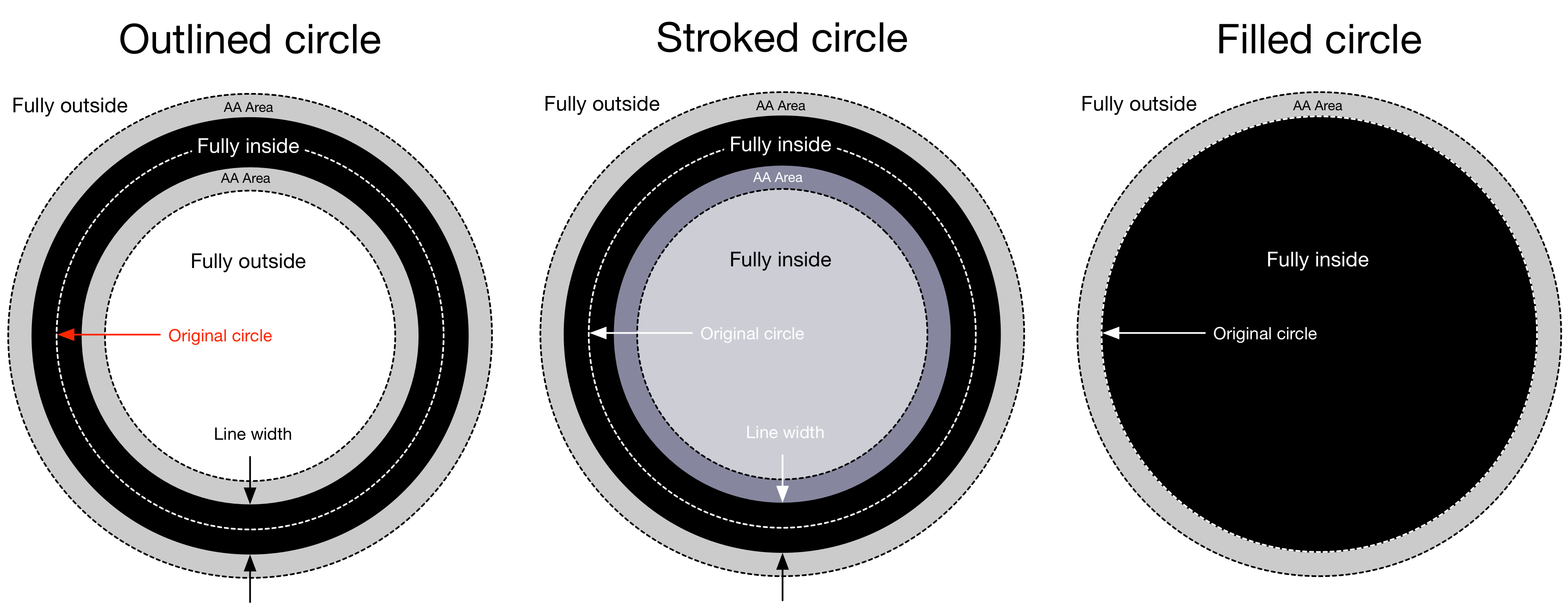
Figure
For all these cases, we need to define the thickness of the antialiased area, (that is, the area where the estimated coverage will go from 0 (outside) to 1 (inside)) and the line thickness for the stroke and outline cases. This means that wen we compute the actual size of the circle, we have to take this into account (2*antialias + linewidth). The antialias area is usually 1.0 pixel. If it is larger, the shape will appear blurry, and it it is too narrow, the shape will have hard egdes. The degenerated case being zero area that results in no antialias at all.
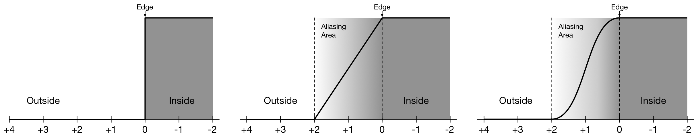
Figure
Finally, we need to define a function that gives the coverage according to the distance. As illustrated above, we have the choice between several solutions (you're also free to design your own) but we'll mostly use the last one for the rest of this book because it appears to be the nicest (to me).
Rendering points
.
If you have read the previous chapters, you may have noticed that there exists
actually a gl.GL_POINTS drawing primitive and you might have concluded (quite
logically) that displaying points in OpenGL is straightforward. This is partly
true. This primitive can be actually used to display points, but the concept of
point for OpenGL is roughly a non-antialiased, non-rotated, boring and ugly
square. Consequently, if we want to display points like in the teaser image
above , we'll need to take care of pretty much everything.
Dots, discs, circles
Raw points
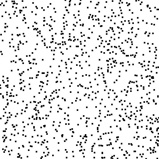
The most straightforward way to display points is to use the gl.GL_POINTS
primitive that displays a quad that is always facing the camera
(i.e. billboard). This is very convenient because a mathematical point has no
dimension, even though we'll use this primitive to draw discs and circles in
the next section. The size of the quad must be specified within the vertex
shader using the gl_PointSize variable (note that the size is expressed in
pixels). As shown on the figure, the result is quite ugly.
import numpy as np
from glumpy import app, gloo, gl

vertex = """
  attribute vec2 position;
  void main() {
      gl_PointSize = 5.0;
      gl_Position = vec4(position, 0.0, 1.0);
  } """

fragment = """
  void main() {
       gl_FragColor = vec4(vec3(0.0), 1.0);
  } """

window = app.Window(512, 512, color=(1,1,1,1))
points = gloo.Program(vertex, fragment, count=1000)
points["position"] = np.random.uniform(-1,1,(len(points),2))

@window.event
def on_draw(dt):
    window.clear()
    points.draw(gl.GL_POINTS)

app.run()
Antialiased points
For drawing antialiased point, the size of the quad must be slighlty larger
than the actual diameter of the point because we need some extra space for the
antialias area. Considering a point with a radius r, the size of the quad is
thus 2+ceil(2*r) if we consider using 1 pixel for the antalias area. Finally,
considering a point centered at center with radius radius, our vertex
shader reads (see also previous chapter on signed distance field):
// Screen resolution as (width, height)
uniform vec2 resolution;

// Point center (in pixel coordinates)
attribute vec2 center;

// Point radius (in pixels)
attribute float radius;

varying vec2 v_center;
varying float v_radius;
void main()
{
    v_radius = radius;
    v_center = center;
    gl_PointSize = 2.0 + ceil(2.0*radius);
    gl_Position = vec4(2.0*center/resolution-1.0, 0.0, 1.0);
}
You may have noticed that we gave the window resolution to the shader using a
uniform (that will be updated each time the window size has changed). The goal
is to be able to use window coordinates (i.e. pixels) from within Python
without taking care of the normalized device coordinate (this transformation
has been done in the vertex shader above). We now have one problem to solve. A
GL point is made from a single vertex and the apparent size of the resulting
quad is controlled by the gl_PointSize variable resulting in several
fragments. How things are interpolated between vertices knowing there is ony
one vertex? The answer is that there is no interpolation. If we want to know
the position of a fragment relatively to the center, we have to find it
ourself. Luckily, there is one interesting variable gl_FragCoord that gives
us the absolute coordinate of the fragment in window coordinates (bottom-left
is (0,0)). Subtracting the center from this coordinate will give us the
relative position of the fragment from which we can compute the distance to the
outer border of the point. Finally, our fragment shader reads:
varying vec2 v_center;
varying float v_radius;
void main()
{
    vec2 p = gl_FragCoord.xy - v_center;
    float a = 1.0;
    float d = length(p) - v_radius;
    if(d > 0.0) a = exp(-d*d);
    gl_FragColor = vec4(vec3(0.0), a);
}
Last, we setup our python program to display some discs:
V = np.zeros(16, [("center", np.float32, 2),
                  ("radius", np.float32, 1)])
V["center"] = np.dstack([np.linspace(32, 512-32, len(V)),
                         np.linspace(25, 28, len(V))])
V["radius"] = 15

window = app.Window(512, 50, color=(1,1,1,1))
points = gloo.Program(vertex, fragment)
points.bind(V.view(gloo.VertexBuffer))

@window.event
def on_resize(width, height):
    points["resolution"] = width, height

@window.event
def on_draw(dt):
    window.clear()
    points.draw(gl.GL_POINTS)

app.run()


You can see the result on the image on the right. Not only the discs are properly antialiased, but they are also positionned at the subpixel level. In the image on the right, each disc is actually vertically shifted upward by 0.2 pixels compared to its left neightbour. However, you cannot see any artefacts (can you?): the discs are similar and properly aligned. For the disc outlines, we simply have to get the absolute distance instead of the signed distance.
varying vec2 v_center;
varying float v_radius;
void main()
{
    vec2 p = gl_FragCoord.xy - v_center;
    float a = 1.0;
    float d = length(p) - v_radius;
    if(abs(d) > 0.0) a = exp(-d*d);
    gl_FragColor = vec4(vec3(0.0), a);
}
Ellipses
Figure
Rendering ellipses is harder than it seems because, as we've explained in a
previous chapter, computing the distance from an arbitrary point to an ellipse
is surprinsingly difficult if you compare it to the distance to a circle. The
second difficulty for us is the fact that an ellipse can be very "flat" and if
we use the gl.GL_POINTS primitive, a lot of useless fragment will be
generated. This is the reason why we need to compute the bounding box
(including thickness and antialias area) and use two triangles to actually
display the ellipse. Last difficulty is that we cannot take advantage of the
gl_FragCoord but we can now take advantage of the four vertices to have local
coordinate interpolation in the fragment shader.
uniform vec2 resolution;
uniform float theta;
attribute vec2 position;
attribute float angle;
varying vec2 v_position;
void main() {
    v_position = position;
    vec2 p = position;
    p = vec2(p.x*cos(angle+theta) - p.y*sin(angle+theta),
             p.y*cos(angle+theta) + p.x*sin(angle+theta));
    p = p + resolution/2.0;
    gl_Position = vec4(2.0*p/resolution-1.0, 0.0, 1.0);
}
Note that in the vertex shader above, we pass the non-rotated coordinates to the fragment shader. It makes things much simpler in the fragment shader that reads:
float SDF_fake_ellipse(vec2 p, vec2 size) {
  float a = 1.0;
  float b = size.x/size.y;
  float r = 0.5*max(size.x,size.y);
  float f = length(p*vec2(a,b));
  return f*(f-r)/length(p*vec2(a*a,b*b));
}

uniform vec2 size;
varying vec2 v_position;
void main() {
    float d = SDF_fake_ellipse(v_position, size) + 1.0;
    float alpha;
    if (abs(d) < 1.0) alpha = exp(-d*d)/ 4.0;
    else if (d < 0.0) alpha =       1.0/16.0;
    else              alpha = exp(-d*d)/16.0;
    gl_FragColor = vec4(vec3(0.0), alpha);
}
Spheres
Flat sphere
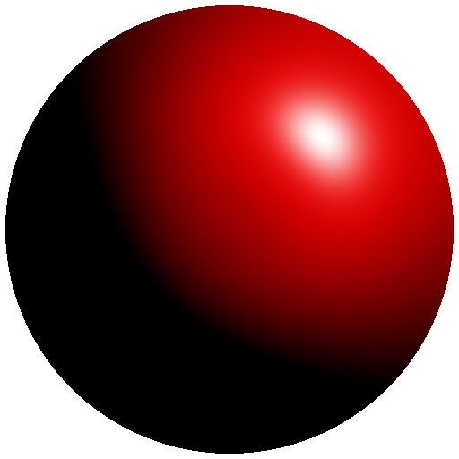
Figure
If you look closely at a sphere, you'll see that that the projected shape on screen is actualy as disc as shown on the figure on the right. This is actually true independently of the viewpoint and we can take advantage of it. A long time ago (with the fixed pipeline), rendering a sphere meant tesselating the sphere with a large number of triangles. The larger the number of triangles, the higher the quality of the sphere and the slower the rendering. However, with the advent of shaders, things have changeg dramatically and we can use fake spheres, i.e. discs thar are painted such as to appear as spheres. This is known as "impostors". If you look again at the image, you might realize that the appeareance of the sphere is given by the shading that is not uniform and suggests instead a specific lighting that seems to come from the upper right corner. Let's see if we can reproduce this.
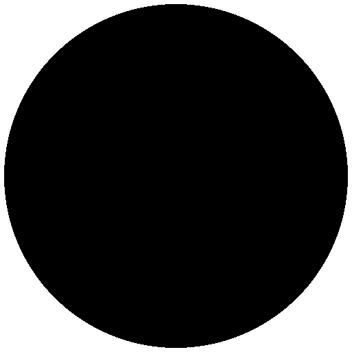
First thing first, Let's setup a scene in order to display a single and large disc. To do that, we simply test if a fragment is inside or outside the circle:
varying vec2 v_center;
varying float v_radius;
void main()
{
    vec2 p = gl_FragCoord.xy - v_center;
    float z = 1.0 - length(p)/v_radius;
    if (z < 0.0) discard;
    gl_FragColor = vec4(vec3(0.0), 1.0);
}
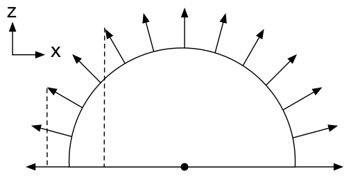
Figure
To simulate lighting on the disc, we need to compute normal vectors over the
surface of the sphere (i.e. disc). Luckily enough for us, computing the normal
for a sphere is very easy. We can simply use the p=(x,y) coordinates inside the
fragment shader and compute the z coordinate. How? you might ask
yourself. This is actually correlated to the distance d to the center such
that z = 1-d. If you want to convice yourself, just look at the figure on
the right that show a side view of half a sphere on the xz plane. The z
coordinate is maximal in the center and null on the border.
We're ready to simulate lighting on our disc using the Phong model. I won't give all the detail now because we'll see that later. However, as you can see on the source below, this is quite easy and the result is flawless.

varying vec2 v_center;
varying float v_radius;
void main()
{
    vec2 p = (gl_FragCoord.xy - v_center)/v_radius;
    float z = 1.0 - length(p);
    if (z < 0.0) discard;

    vec3 color = vec3(1.0, 0.0, 0.0);
    vec3 normal = normalize(vec3(p.xy, z));
    vec3 direction = normalize(vec3(1.0, 1.0, 1.0));
    float diffuse = max(0.0, dot(direction, normal));
    float specular = pow(diffuse, 24.0);
    gl_FragColor = vec4(max(diffuse*color, specular*vec3(1.0)), 1.0);
}
True sphere
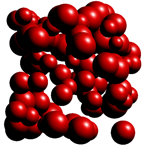
Figure
We can use this technique to display several "spheres" having different sizes
and positions as shown on the figure on the right. This can be used to
represent molecules for examples. Howewer, we have a problem with sphere
intersecting each other. If you look closely the figure, you might have notices
that no sphere intersect any sphere. This is due to the depth testing of the
unique vertex (remember gl.GL_POINTS) that is used to generate the quad
fragments. Each of these fragments share the same z coordinate resulting in
having sphre fully in front of another of fully behind another. For accurate
rendering, we thus have to tell OpenGL what is the depth of each fragment using
the gl_FragDepth variable (that must be between 0 and 1):
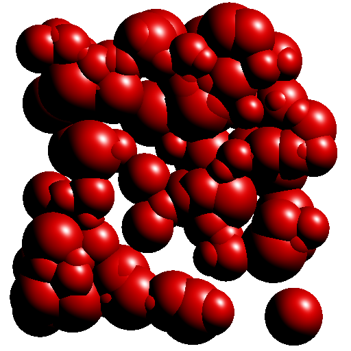
varying vec3 v_center;
varying float v_radius;
void main()
{
    vec2 p = (gl_FragCoord.xy - v_center.xy)/v_radius;
    float z = 1.0 - length(p);
    if (z < 0.0) discard;

    gl_FragDepth = 0.5*v_center.z + 0.5*(1.0 - z);

    vec3 color = vec3(1.0, 0.0, 0.0);
    vec3 normal = normalize(vec3(p.xy, z));
    vec3 direction = normalize(vec3(1.0, 1.0, 1.0));
    float diffuse = max(0.0, dot(direction, normal));
    float specular = pow(diffuse, 24.0);
    gl_FragColor = vec4(max(diffuse*color, specular*vec3(1.0)), 1.0);
}
You can see on the figures that the spheres now intersect each other correctly.
Exercises
Tiny discs
Figure
Adapting the shader from the "Dots, discs, circles" section, try to write a script to draw discs on a spiral as displayed on the figure on the right. Be careful with small discs, especially when the radius is less than one pixel. In such case, you'll have to find a convincing way to suggest the size of the disc...
Solution: spiral.py
Antialiased triangles
Figure
Try to adapt the code from the ellipses section to remake the animation on the right. Be careful with the computation of the bouding box.
Solution: triangles.py
GPU Voronoi
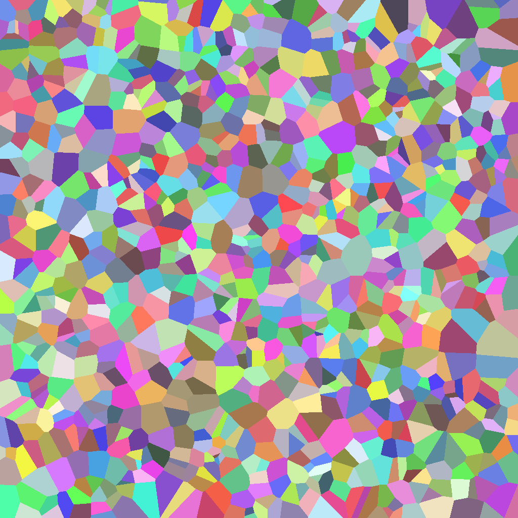
Figure
We've seen when rendering sphere that the individual depth of each fragment can be controled withing the fragment shader and we computed this depth by taking the distance to the center of each disc/sphere. The goal of this exercise is thus to adapt this method to render a Voronoi diagram as shown on the right.
Solution: voronoi.py
Rendering markers
Markers and arrows are important components in scientific visualisation. Markers help to visualize individual points and aggregated data while arrows can be used to visualize a stream flow. Markers and arrows can be actually rendered very fast by taking advantage of the shader. In fact, they can be drawn entirely inside the shader provided we know the size, the type and the orientation. The teaser figure comes from an article I wrote and published in the journal of Computer Graphics and Techniques. The content of this chapter is largely inspired by this article.
Constructive Solid Geometry
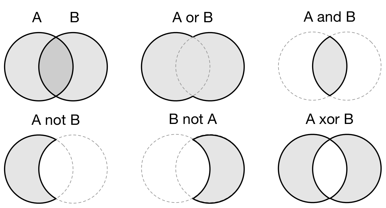
Figure
Constructive solid geometry (CSG) is a technique used for modeling in order to create a complex object by using Boolean operators to combine simpler objects (primitives). Resulting objects appear visually complex but are actually a cleverly combined or decombined objects. The teaser image in the GLSL References chapter is the result of complex constructive geometry in 3D. See also the Wikipedia entry on Truth function.
This is the reason we did not bother to try to render complex shapes in the previous section. Using constructive solid geometry, we are free to model pretty much anything and we'll see that in the markers section below. In the meantime, we need to define our CSG operations in glsl. The good news is that it is incredibly simple, just read:
// Union (A or B)
float csg_union(float d1, float d2)
{ return min(d1,d2); }

// Difference (A not B)
float csg_difference(float d1, float d2)
{ return max(d1,-d2); }

// Intersection (A and B)
float csg_intersection(float d1, float d2)
{  return max(d1,d2); }

// Exclusion (A xor B)
float csg_exclusion(float d1, float d2)
{ return min(max(d1,-d2), max(-d1,d2)); }
And we can check for the result using two circles (the shadertoy link for each example allows you to play online with them):
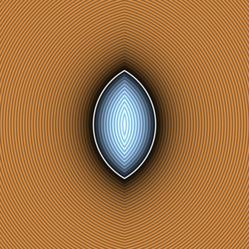
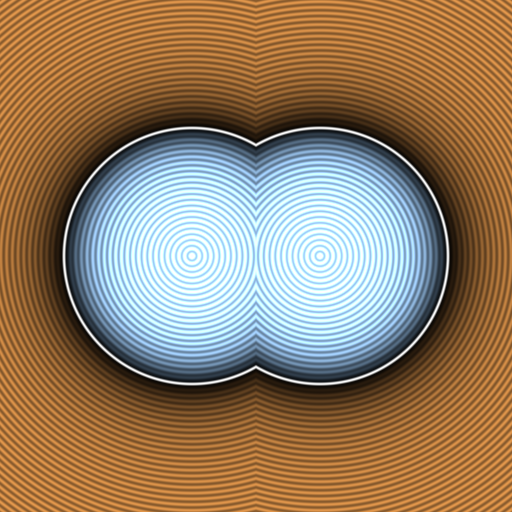
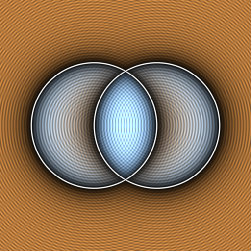
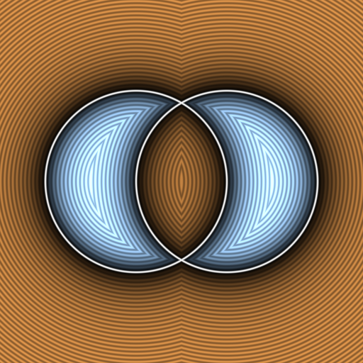
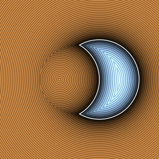
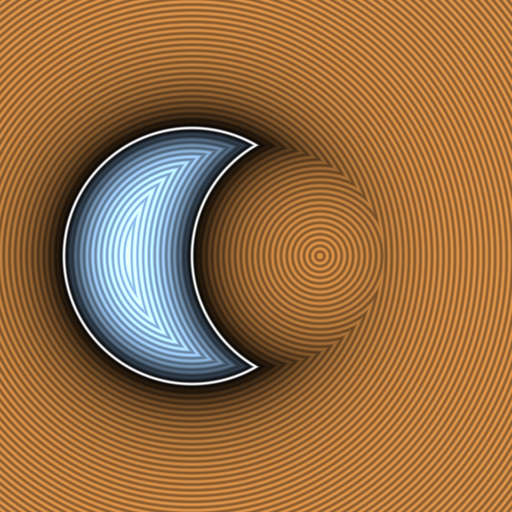
Markers
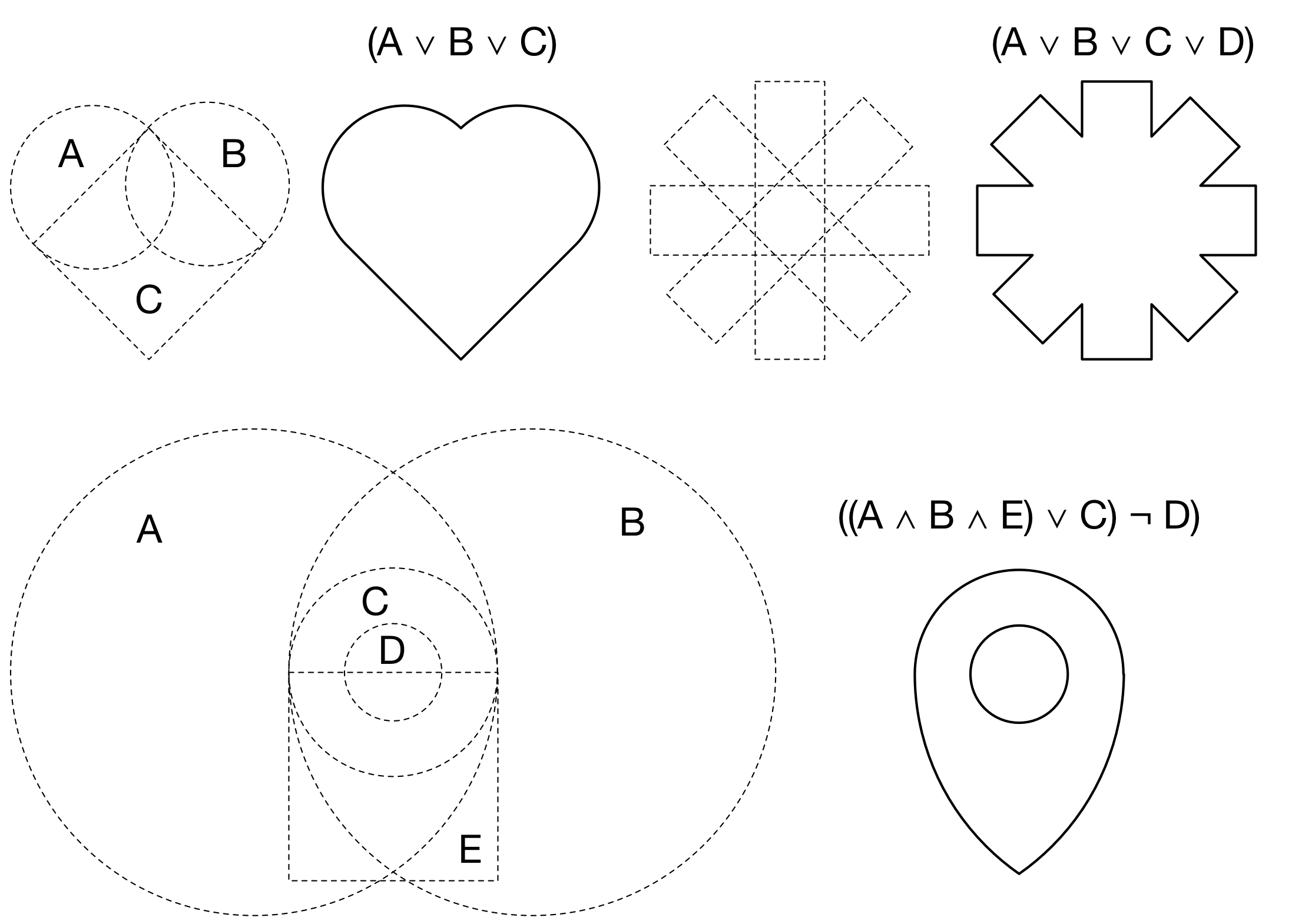
Figure
As illustrated on the right figure creating markers is merely a matter of imagination. Try to think of a precise shape and see how you can decompose it in terms of constructive solid geometry. I've put a collection of such markers in the (open access) article Antialiased 2D Grid, Marker, and Arrow Shaders.
All these markers are also defined in the glumpy library. Have a look at the marker.py example where you can experiment with the different markers and the different rendering options. Feel free to design your own and to open a pull request to have them added to glumpy. Note that all the markers have a default orientation that can be changed very easily from within the shader.
For example, the heart marker, which is made of two discs and one sphere, reads as follows:
float marker_heart(vec2 P, float size)
{
   float x = M_SQRT2/2.0 * (P.x - P.y);
   float y = M_SQRT2/2.0 * (P.x + P.y);

   // Square
   float r1 = max(abs(x),abs(y))-size/3.5;

   // Disc 1
   float r2 = length(P - M_SQRT2/2.0*vec2(+1.0,-1.0)*size/3.5) - size/3.5;

   // Disc 2
   float r3 = length(P - M_SQRT2/2.0*vec2(-1.0,-1.0)*size/3.5) - size/3.5;

   return min(min(r1,r2),r3);
}
Figure
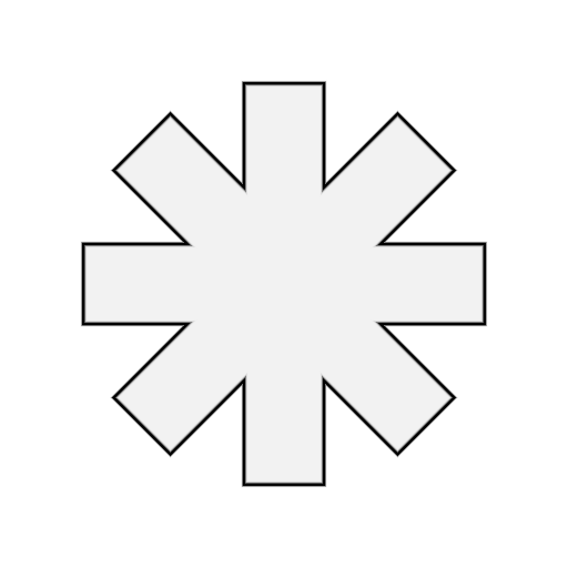
Figure
Figure
Figure
Figure
Figure
Figure
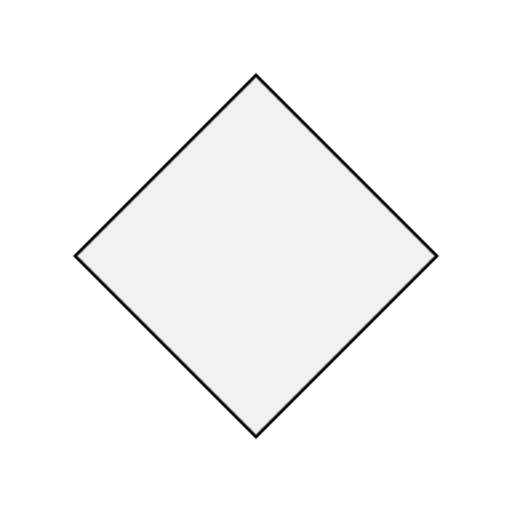
Figure
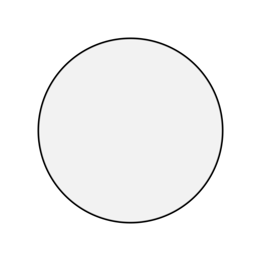
Figure
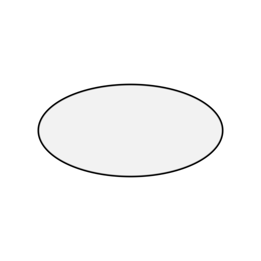
Figure
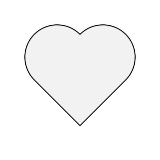
Figure
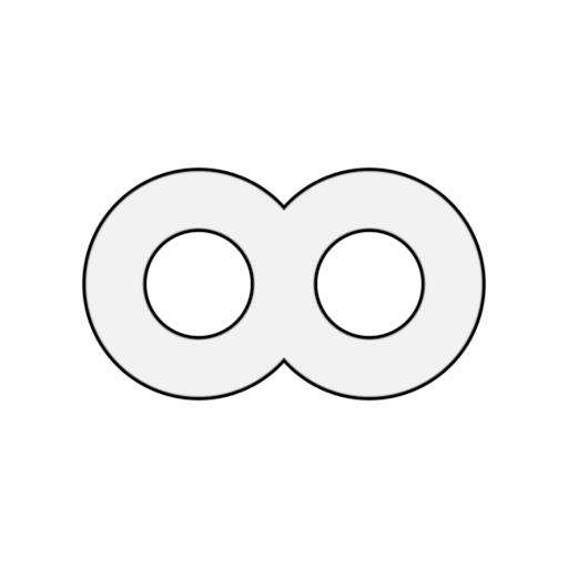
Figure

Figure
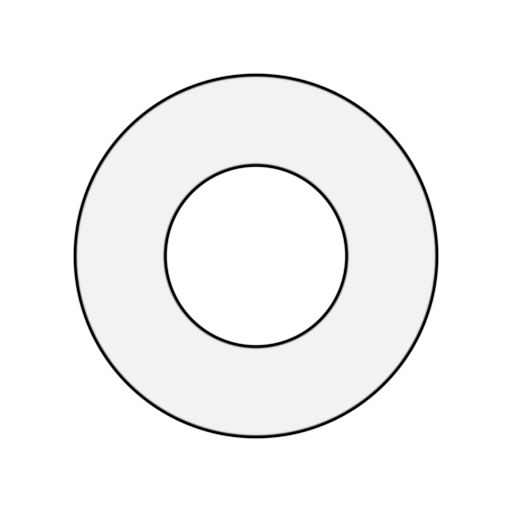
Figure
Figure
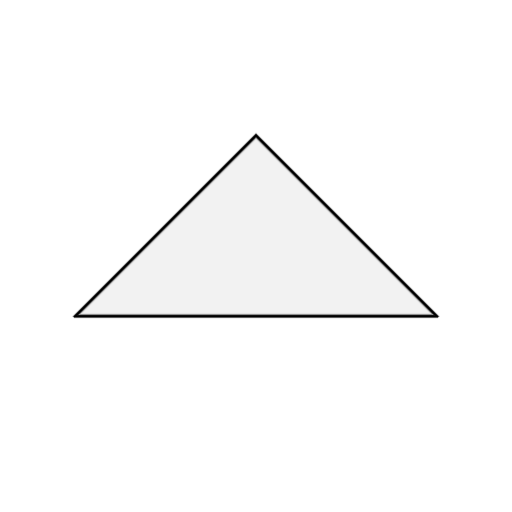
Figure
Arrows
Arrows are a bit different from markers because they are made of a body, which is a line basically, and a head. Most of the difficulty lies in the head definition that may vary a lot depending on the type the arrow. For example, the stealth arrow shader reads:
float line_distance(vec2 p, vec2 p1, vec2 p2) {
    vec2 center = (p1 + p2) * 0.5;
    float len = length(p2 - p1);
    vec2 dir = (p2 - p1) / len;
    vec2 rel_p = p - center;
    return dot(rel_p, vec2(dir.y, -dir.x));
}

float arrow_stealth(vec2 texcoord,
                    float body, float head,
                    float linewidth, float antialias)
{
    float w = linewidth/2.0 + antialias;
    vec2 start = -vec2(body/2.0, 0.0);
    vec2 end   = +vec2(body/2.0, 0.0);
    float height = 0.5;

    // Head : 4 lines
    float d1 = line_distance(texcoord, end-head*vec2(+1.0,-height),
                                       end);
    float d2 = line_distance(texcoord, end-head*vec2(+1.0,-height),
                                       end-vec2(3.0*head/4.0,0.0));
    float d3 = line_distance(texcoord, end-head*vec2(+1.0,+height), end);
    float d4 = line_distance(texcoord, end-head*vec2(+1.0,+0.5),
                                       end-vec2(3.0*head/4.0,0.0));

    // Body : 1 segment
    float d5 = segment_distance(texcoord, start, end - vec2(linewidth,0.0));

    return min(d5, max( max(-d1, d3), - max(-d2,d4)));
}
Glumpy provides 8 types of arrows that you can see below. You can also have a look at the arrow.py example where you can experiment with the different shapes and rendering options. Feel free to design your own and to open a pull request to have them added to glumpy.
Figure
Figure
Figure
Figure
Figure
Figure
Figure
Figure
Texture based

Figure
We've seen that constructive solid geometry is a powerful tool for the design of quite complex shapes. It is also very fast since everything is computed on the GPU. Of course, the more complex is the shape, the slower it will be to evaluate and thus to render. However, for really complex shapes, it might not be possible to express the shape in mathematical terms and we have to find another way. The idea is to actually precompute the signed distance to an arbitrary shape on the CPU and to store the result in a texture.
This computation quite be quite intensive and this the reason why it is preferable to code it in C. Glumpy comes with the binding for the "Anti-Aliased Euclidean Distance Transform" method proposed by Stefan Gustavson and Robin Strand.

Figure
If you run the code below, you should obtain the image on the right.
import numpy as np
from PIL import Image
from glumpy.ext.sdf import compute_sdf

Z = np.array(Image.open("firefox.png"))
compute_sdf(Z)
image = Image.fromarray((Z*255).astype(np.ubyte))
image.save("firefox-sdf.png")
Even though the logo is barely recognisable on the resulting image, it carries nonetheless the necessary information to compute the distance to the border from within the shader. When the texture will be read inside the fragment shader, we'll subtract 0.5 from the texture value (texture value are normalized, hence the 0.5) to obtain the actual signed distance field. You're then free to use this distance for accurate rendering of your shape. Needless to say that the precision of the distance is directly correlated with the size of your texture...
Figure
The fragment shader reads (see also texture-marker.py):
varying float v_size;
varying vec2 v_texcoord;
uniform float linewidth;
uniform float antialias;
uniform sampler2D texture;
void main() {
    float size = v_size + linewidth + 2.0*antialias;
    float signed_distance = size*(texture2D(texture, v_texcoord).r - 0.5);
    float border_distance = abs(signed_distance) - linewidth/2.0 + antialias;
    float alpha = border_distance/antialias;
    alpha = exp(-alpha*alpha);
    if (border_distance < 0)
        gl_FragColor = vec4(0.0, 0.0, 0.0, 1.0);
    else if (border_distance < (linewidth/2.0 + 2.0*antialias))
        gl_FragColor = vec4(0.0, 0.0, 0.0, alpha);
    else
        discard;
}
Exercises
Quiver plot
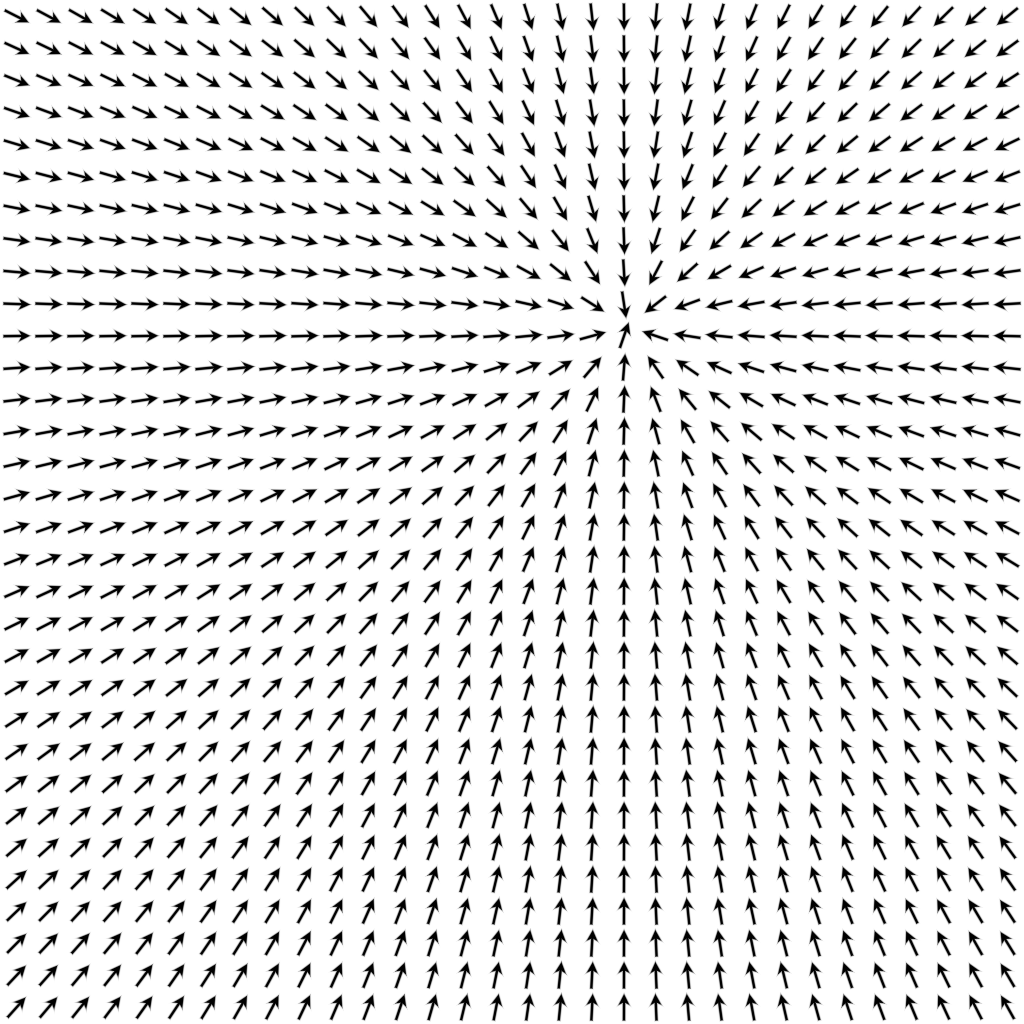
Figure
Now that we know how to draw arrows, we can make a quiver plot very easily. The obvious solution would be to draw n arrows using 2×n triangles (since one arrow is two triangle). However, if your arrows are evenly spaced as on the figure on the right, there is a smarter solution using only two triangles.
Solution: quiver.py
Light and shadows
Figure
As explained before, the shadertoy website is a great resource and you can learn a lot by reading the sources accompanying each demo. As an exercise, have a look at this wonderful demo by Marteen that shows two dimensional signed distance field functions with light and shadows.
Simply gorgeous...
Rendering lines
.
Lines are most certainly among the most important components in scientific visualization. They can be used to represents axis, frames, plots, error bars, contours, grids, etc. Lines and segments are among the most simple geometrical objects. And yet, they can become quite complex if we consider line thickness, cap, joint and pattern such as dotted, dashed, etc. In the end, rendering lines with perfect quality is a lot of work as you'll read below. But it's worth the effort as illustrated in the teaser image above. This comes from an interactive demo of glumpy (See the spiral demo).
Raw Lines
As we've seen in the Quickstart chapter, OpenGL come with three different line
primitives, namely gl.GL_LINES (segments), gl.GL_LINE_STRIP (polyline) and
gl.GL_LINE_LOOP (closed polyline) and correspond to the hardware
implementation of the Bresenham algorithm that can be
written as:
def line(x0, y0, x1, y1, image, color):
    steep = False
    if abs(x0-x1) < abs(y0-y1):
        x0, y0 = y0, x0
        x1, y1 = y1, x1
        steep = True
    if x0 > x1:
        x0, x1 = x1, x0
        y0, y1 = y1, y0
    dx = x1-x0
    dy = y1-y0
    error2 = 0
    derror2 = abs(dy)*2
    y = y0
    for x in range(x0,x1+1):
        if steep:
            set_pixel(image, y, x, color)
        else:
            set_pixel(image, x, y, color)
        error2 += derror2;
        if error2 > dx:
            y += 1 if y1 > y0 else -1
            error2 -= dx*2
Rendering raw lines using OpenGL is incredibly fast. Really, really fast. This means that it can be used for the rendering of real-time signals as we'll see in the exercises section.
But as you may have guessed by now, the result is also really, really ugly because these lines are not antialiased and cannot be wider than 1 pixel. Click on the image on the right if you want to see it. But you've be warned. It makes my eyes bleed each time I look at it.
Segments
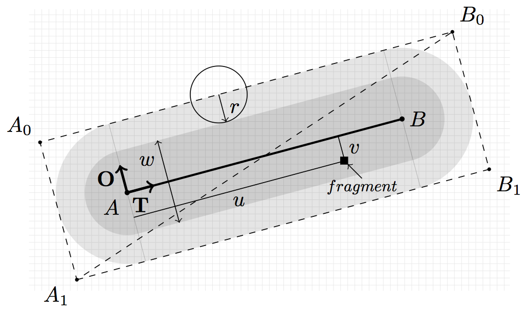
Figure
If we want to render nice lines, we'll have to draw triangles...
More precisely, we need two triangle for a thick (or thin it doesn't really matter) line segment. The idea is to compute the signed distance to the segment envelope like we did in the previous section for markers. However, we have a supplementary difficulty because we also need to draw segment caps as illustrated on the figure on the right. This means that when we generate our triangles, we have to take into account antialias area and the cap size (half the line thickness for one cap).
Let us consider a segment AB and let us name T the tangent to AB and O
the normal to AB. We want to draw a segment of thickness w using an
antialias area (filter radius) r. From these information, we can compute the
4 necesssary vertices (screen space (x,y)):
A₀ = A - (w/2 + r) * (T+O)A₁ = A - (w/2 + r) * (T-O)B₀ = B + (w/2 + r) * (T+O)B₁ = B + (w/2 + r) * (T-O)
We can also parameterize these four vertices using a local frame reference
where the origin is A and the direction is horizontal (see figure above):
A₀/(u,v) = ( -w/2-r, +w/2-r)A₁/(u,v) = ( -w/2-r, -w/2-r)B₀/(u,v) = (|AB| + w/2-r, +w/2-r)B₁/(u,v) = (|AB| + w/2-r, -w/2-r)
This parameterization is very convenient because the distance to the segment
body is given by the v component while the cap areas can be identified using
u < 0 or x > |AB|.
The next question is where do we compute all these information? We could do it
at the python level of course but it would be slower than computing directly
within the shader. So let's do that instead. For this, we need to distinguish
between each vertex and we need to compute T and O, meaning each vertex
needs an access to A, B and a unique identifier to know wheter we're dealing
with A₀, A₁, B₀ or B₁.
A₀: A, B, (u,v) = (0,1)A₁: A, B, (u,v) = (0,0)B₀: A, B, (u,v) = (1,1)B₁: A, B, (u,v) = (1,0)
From this information, we can now compute each vertex position Pᵢ and
parameterization UVᵢ;
T = (B-A)/|AB|
O = (-T.y, T.x)
Pᵢ = A + u*T*|AB| + (2*u-1)*T*(w/2 + r) + (2*v-1)*O*(w/2 + r)
T = i
O = j
UVᵢ = u*T*|AB| + (2*u-1)*T*(w/2 + r) + (2*v-1)*O*(w/2 + r)
Translated in shader code, that gives us:
uniform vec2 resolution;
uniform float antialias;
attribute float thickness;
attribute vec2 p0, p1, uv;
void main() {
    float t = thickness/2.0 + antialias;
    float l = length(p1-p0);
    float u = 2.0*uv.x - 1.0;
    float v = 2.0*uv.y - 1.0;

    // Screen space
    vec2 T = normalize(p1-p0);
    vec2 O = vec2(-T.y , T.x);
    vec2 p = p0 + uv.x*T*l + u*T*t + v*O*t;
    gl_Position = vec4(2.0*p/resolution-1.0, 0.0, 1.0);

    // Local space
    T = vec2(1.0, 0.0);
    O = vec2(0.0, 1.0);
    p = uv.x*T*l + u*T*t + v*O*t;
In the fragment shader, we can then use the local coordinate to decide on the color to be rendered by computing the signed distance to the envelope.
uniform float antialias;
varying float v_thickness;
varying vec2 v_p0, v_p1, v_p;
void main() {
    float d = 0;
    if( v_p.x < 0 )
        d = length(v_p - v_p0) - v_thickness/2.0 + antialias/2.0;
    else if ( v_p.x > length(v_p1-v_p0) )
        d = length(v_p - v_p1) - v_thickness/2.0 + antialias/2.0;
    else
        d = abs(v_p.y) - v_thickness/2.0 + antialias/2.0;
    if( d < 0)
        gl_FragColor = vec4(0.0, 0.0, 0.0, 1.0);
    else if (d < antialias) {
        d = exp(-d*d);
        gl_FragColor = vec4(0.0, 0.0, 0.0, d);
    }
The actual shader is slightly more complicated because we have also to take care of lines whose thickness is below 1 pixel. In such a case, we consider the line to be one pixel wide and we use transparency level to suggest that the line is actually thiner. If you look at the result below (see agg-segments.py), the first few lines have a thickness below 1 pixel.
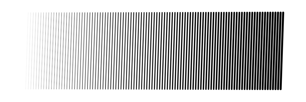
Figure
Concerning the segment caps, we have used a round cap, but you're free to use any cap you like. In fact, you could have used any marker we've seen in the previous chapter or no caps at all (just discard the fragment in such case).
Lines
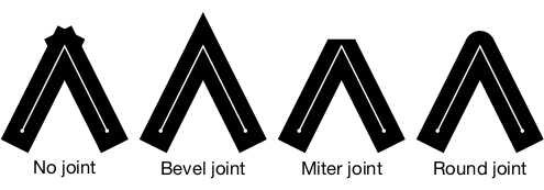
Figure
Polylines (i.e. line made of several segments) is much more difficult to render than segment because we have to take joints into account as illustrated on the image on the right. But, even if there appears to exist three different kind of joints, there are really only two cases to consider: the bevel joint and the others (round and miter). These cases are different because we can code a reasonably fast solution for the bevel case while the two others ask for more work. This is important because for smooth lines, such as Bézier curves (see below), the fast solution will do the job.
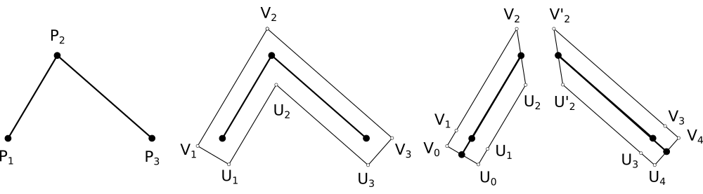
Figure
The reason the fast solution is fast compared to the other one comes from the number of vertices we need to generate to render a thick line. In the fast case, we'll need only 2×n vertices while in the other, we'll need 4×n vertices (and a lot of tests inside the shader).
Smooth lines
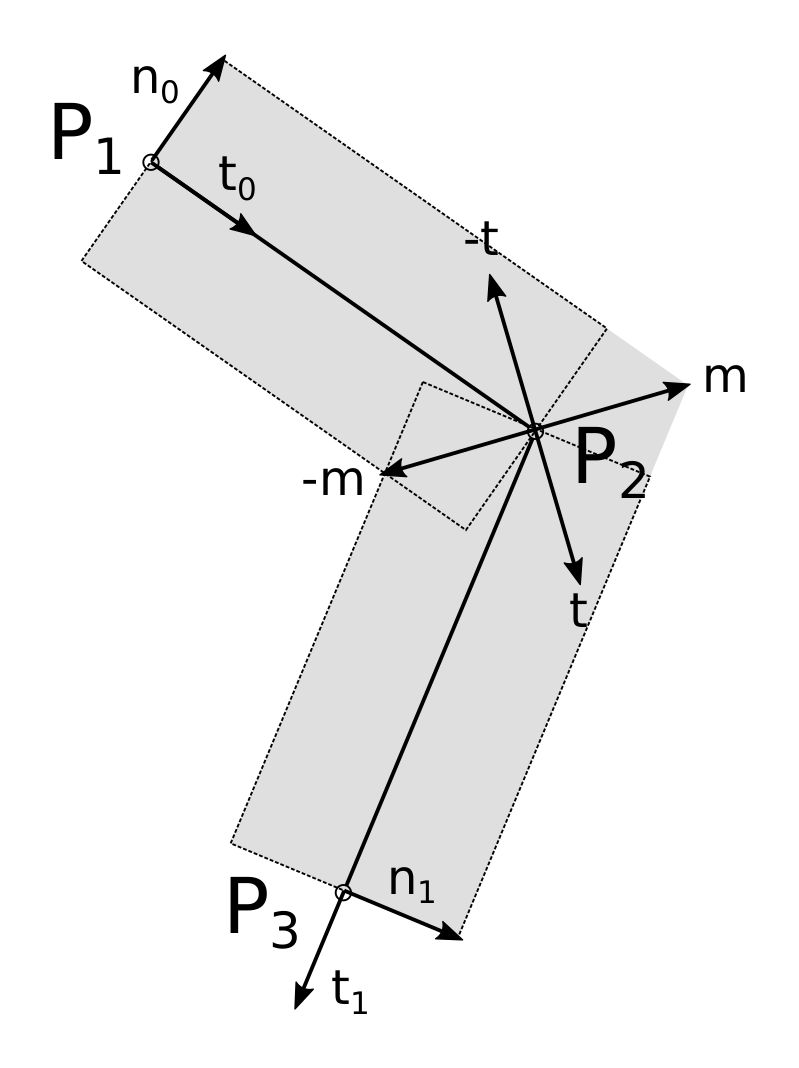
Figure
In order to compute the final position of a vertex inside the vertex shader, we
need to have access to the previous and the next vertex as shown on the figure
on the right. To compute m at P₂ we need to have access to P₁ and
P₃. Furthermore, each vertex needs to be doubled and we need to take care of
line start and end. To do that, we'll use a single vertex buffer that is baked
such that we each vertex is doubled and two extra vertices are put at start and
end:
┌───┬───┬───┬───┬───┬───┬───┬───┬───┬───┐
│ 0 │ 0 │ 1 │ 2 │ 3 │ 4 │ 5 │ 6 │ 7 │ 7 │
└───┴───┴───┴───┴───┴───┴───┴───┴───┴───┘

└──────────── prev ─────────────┘

    └──────────── curr ─────────────┘

        └──────────── next ─────────────┘
The goal of these two extra vertices is to use the same buffer for passing the
prev, curr and next attributes to the vertex shader using the same
underlying buffer. Their content will depend on whether the line is closed or
not. It is to be noted that each vertex has four coordinates. The (x,y) gives
the actual vertex coordinates, the z=+1/-1 coordinate identifies which vertex
we're dealing with (Vᵢ or Uᵢ on the figure) and the last coordinate is the
curvilinear coordinate along the line. This last one will be useful to know if
we're within the start cap area, the end cap area or inside the
body. Furthermore, it can be used for pattern or texturing (see section
Patterns below).
Taking all these constraints into account, the line preparation reads:
def bake(P, closed=False):
    epsilon = 1e-10
    n = len(P)
    if closed and ((P[0]-P[-1])**2).sum() > epsilon:
        P = np.append(P, P[0])
        P = P.reshape(n+1,2)
        n = n+1
    V = np.zeros(((1+n+1),2,4), dtype=np.float32)
    V_prev, V_curr, V_next = V[:-2], V[1:-1], V[2:]
    V_curr[...,0] = P[:,np.newaxis,0]
    V_curr[...,1] = P[:,np.newaxis,1]
    V_curr[...,2] = 1,-1
    L = np.cumsum(np.sqrt(((P[1:]-P[:-1])**2).sum(axis=-1))).reshape(n-1,1)
    V_curr[1:,:,3] = L
    if closed:
        V[0], V[-1] = V[-3], V[2]
    else:
        V[0], V[-1] = V[1], V[-2]
    return V_prev, V_curr, V_next, L[-1]
Using this baking, it is now realtively easy to compute vertex position from within the vertex shader. The only difficulty being to parameterize properly the vertex such as to have all information to perform the antialiasing inside the fragment shader:
uniform vec2 resolution;
uniform float antialias, thickness, linelength;
attribute vec4 prev, curr, next;
varying vec2 v_uv;

void main() {
    float w = thickness/2.0 + antialias;
    vec2 p;
    vec2 t0 = normalize(curr.xy - prev.xy);
    vec2 t1 = normalize(next.xy - curr.xy);
    vec2 n0 = vec2(-t0.y, t0.x);
    vec2 n1 = vec2(-t1.y, t1.x);

    // Cap at start
    if (prev.xy == curr.xy) {
        v_uv = vec2(-w, curr.z*w);
        p = curr.xy - w*t1 + curr.z*w*n1;
    // Cap at end
    } else if (curr.xy == next.xy) {
        v_uv = vec2(linelength+w, curr.z*w);
        p = curr.xy + w*t0 + curr.z*w*n0;
    // Body
    } else {
        vec2 miter = normalize(n0 + n1);
        float dy = w / dot(miter, n1);
        v_uv = vec2(curr.w, curr.z*w);
        p = curr.xy + dy*curr.z*miter;
    }
    gl_Position = vec4(2.0*p/resolution-1.0, 0.0, 1.0);
}
Adn the fragment shader reads:
uniform float antialias, thickness, linelength;
varying vec2 v_uv;

void main() {
    float d = 0;
    float w = thickness/2.0 - antialias;
    // Cap at start
    if (v_uv.x < 0)
        d = length(v_uv) - w;
    // Cap at end
    else if (v_uv.x >= linelength)
        d = length(v_uv - vec2(linelength,0)) - w;
    // Body
    else
        d = abs(v_uv.y) - w;

    if( d < 0) {
        gl_FragColor = vec4(0.0, 0.0, 0.0, 1.0);
    } else {
        d /= antialias;
        gl_FragColor = vec4(0.0, 0.0, 0.0, exp(-d*d));
    }
}
Note
Note that we'll be using the GL_TRIANGLE_STRIP even though it would be better to use GL_TRIANGLES and to compute the relevant indices. But I feel lazy right now.
Putting it all together, we can draw some nice and smooth lines (see
linestrip.py). Note that for closed lines
such as the star below, first and last vertex needs to be the same (but it is
taken care of in the bake function).
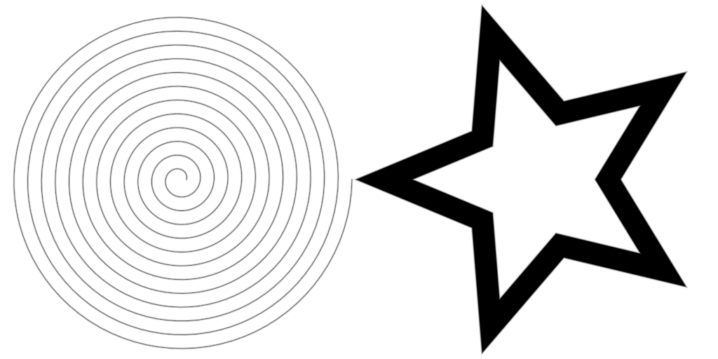
Broken lines
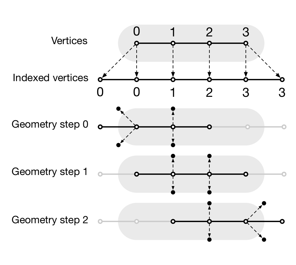
Figure
Broken lines are a bit more difficult because we need a different tesselation just to be able to handle miter and round joints properly in the fragment shader. To be able to do this, we need to know from within the fragment shader if a given fragment is inside the joint area or not. This requires a specific parameterization that relies on having a different tesselation with 4×n vertices instead of 2×n. I won't explain all the details here but only provide the final result that you can found in geom-path.py.
If you look at the sources, you'll see I'm using a geometry shader, which is a
new type of shader that is not officially available in GL ES 2.0 but which is
nonetheless available on a wide number of implementations. This geometry shader
offers the possibility to create new vertex which is quite convenient in our
case because for each couple of vertices we send to the GPU, the geometry
shader will actually create four vertices (see figure above). We thus save the
CPU time of "quadrupling" vertices as we did in the previous section. To be
able to this, we have to use gl.GL_LINES_ADJACENCY_EXT and indicate OpenGL
we'll generate four vertices at each stage, just before the vertex shader:
geometry = gloo.GeometryShader(geometry, 4,
                               gl.GL_LINES_ADJACENCY_EXT,
                               gl.GL_TRIANGLE_STRIP)
Inside the geometry shader, we now have access to four consecutive vertices (in the sense of the provided indices) that can be used to compute the actual position of a given segment of the line. During rendering, we also have to use the same primitives:
@window.event
def on_draw(dt):
    window.clear()
    program.draw(gl.GL_LINE_STRIP_ADJACENCY_EXT, I)
I won't further describe the method that is a bit complicated but you can all the details in the provided demo script. See the caption of the image below.

Bézier curves
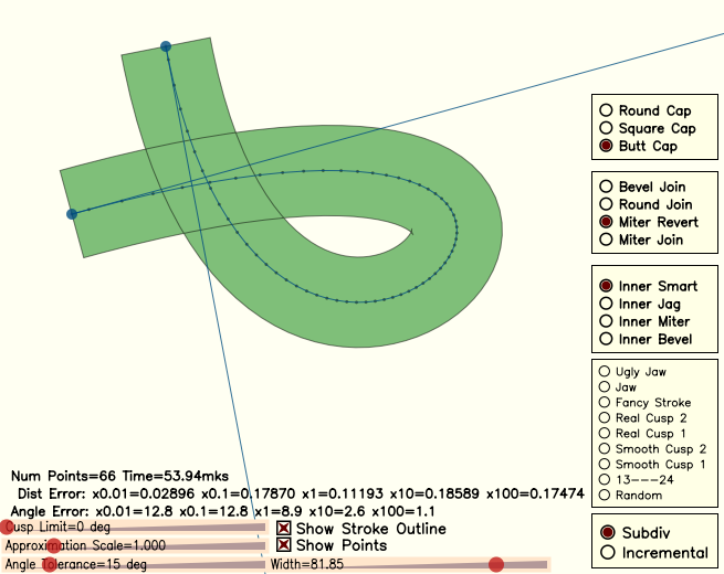
There is a huge litterature on Bézier curves and a huge litterature on GPU Bézier curves as well (+ lot of patents). I won't explain everything here because it would require a whole book and I'm not sure I understand every aspect anyway. If you're interested in the topic, you can have a look at A Primer on Bézier curves by Mike Kamermans (Pomax) that explain pretty much everything but GPU implementation. For GPU implementation, you can have a look at shadertoy and do a search using the "Bézier" or "bezier" keyword (I even commited one myself).
For the time being, we'll use an approximation of Bézier curves using an adaptive subdivision as designed by Maxim Shemarev (and translated in Python by me, see curves.py). You can see on the images below that this method provides a very good approximation in a reasonable number of segments (third figure on the right).
Figure
Figure
Figure
Consequently, for drawing a Bézier curve, we just need to approximate as line segments, bake those segments and render them as shown below (using bevel joint, see bezier.py):

Figure
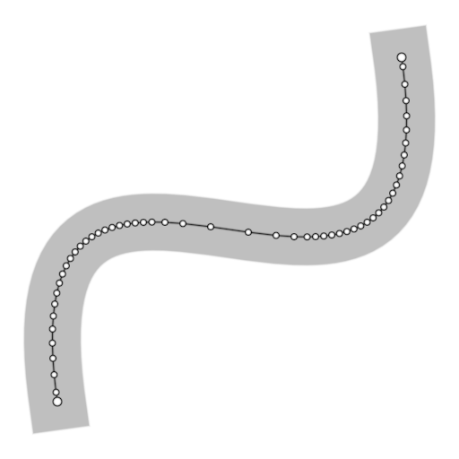
Figure
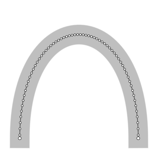
Figure
Patterns
Simple dotted pattern
Figure
Rendering a simple dotted pattern is surprinsingly simple. If you look at the fragmen code from the smooth line sections, the computation of the signed distance reads:
...
// Cap at start
if (v_uv.x < 0)
    d = length(v_uv) - w;
// Cap at end
else if (v_uv.x >= linelength)
    d = length(v_uv - vec2(linelength,0)) - w;
// Body
else
    d = abs(v_uv.y) - w;
...
We can slightly change this code in order to compute the signed distance to discs whose centers area spread over the whole. Do you remember that we took care of computing the line curvilinear coordinate? Having centers spread along this line is then just a matter of a modulo.
uniform float phase;
...
float spacing = 1.5;
float center = v_uv.x + spacing/2.0*thickness
             - mod(v_uv.x + phase + spacing/2.0*thickness, spacing*thickness);
// Discard uncomplete dot at the end of the line
if (linelength - center < thickness/2.0)
    discard;
// Discard uncomplete dot at the start of the line
else if (center < thickness/2.0)
    discard;
else
    d = length(v_uv - vec2(center,0.0)) - w;
...
Figure
The animation is obtained by slowly increasing the phase that makes all dot centers to move along the lines.
By the way, you may have noticed that I've been using the simplest marker I could think of (disc) for the example above. But we could have used any of the marker from the previous chapter actually. For example, on the figure on the right, I use the spade marker and I've added a fading at line start and end to prevent the sudden apparition/disparition of a marker.
Arbitrary dash patterns
Having arbitrary dashed patterns with possibly very thick lines and arbitrary joints is quite a difficult problem if we want to have an (almost) pure GPU implementation. It is actually so hard that I had to write an article explaining how this can be done. If you want to know more, just read See "Shader-based Antialiased Dashed Stroke Polylines" for a full explanation as well as Python implementation. The result is illustrated on the movies below.
Figure
Figure
Figure
Unfortunately, at the time of writing, these arbitrary dash patterns lines have not yet been implemented in glumpy. You're thus more than welcome to make a PR. Contact me if you're interested.
3D lines
Figure
You certainly have noticed that until now, we've been dealing only with lines
in the two-dimensional screen space, using two-dimensional coordinates (x,y)
to describe positions. The thickness of such lines is rather intuitive because
they live in the screen space.
In three dimensions however, the problem is different. Mathematically, a line has no thickness per se and the thick lines we've been drawing so far were actually ribbon. In 3D, we have the choice to consider a thick line to be a ribbon or a tube. But there is actually a third, and simpler option, which is to consider than the line is a ribbon that is always facing the camera.
Fixed apparent thickness
For a fixed apparent thickness, the method is (almost) straighforward:
- Apply transformation and get NDC coordinates
- Convert NDC coordinates to viewport coordinates
- Thicken line in viewport space
- Transmit the resulting vertex
Let's start with the conversion from NDC (normalized device coordinates) to screen:
uniform vec2 viewport;
uniform mat4 model, view, projection;
attribute vec3 prev, curr, next;

...

// Normalized device coordinates
vec4 NDC_prev = projection * view * model * vec4(prev.xyz, 1.0);
vec4 NDC_curr = projection * view * model * vec4(curr.xyz, 1.0);
vec4 NDC_next = projection * view * model * vec4(next.xyz, 1.0);

// Viewport (screen) coordinates
vec2 screen_prev = viewport * ((NDC_prev.xy/NDC_prev.w) + 1.0)/2.0;
vec2 screen_curr = viewport * ((NDC_curr.xy/NDC_curr.w) + 1.0)/2.0;
vec2 screen_next = viewport * ((NDC_next.xy/NDC_next.w) + 1.0)/2.0;
From these screen coordinates, we can compute the final position as we did
previously with the noticeable difference that we also need to use z
coordinate from the NDC coordinate.
vec2 position;
float w = thickness/2.0 + antialias;
vec2 t0 = normalize(screen_curr.xy - screen_prev.xy);
vec2 n0 = vec2(-t0.y, t0.x);
vec2 t1 = normalize(screen_next.xy - screen_curr.xy);
vec2 n1 = vec2(-t1.y, t1.x);
v_uv = vec2(uv.x, uv.y*w);
if (prev.xy == curr.xy) {
    v_uv.x = -w;
    position = screen_curr.xy - w*t1 + uv.y*w*n1;
} else if (curr.xy == next.xy) {
    v_uv.x = linelength+w;
    position = screen_curr.xy + w*t0 + uv.y*w*n0;
} else {
    vec2 miter = normalize(n0 + n1);
    // The max operator avoid glitches when miter is too large
    float dy = w / max(dot(miter, n1), 1.0);
    position = screen_curr.xy + dy*uv.y*miter;
}

// Back to NDC coordinates
gl_Position = vec4(2.0*position/viewport-1.0, NDC_curr.z/NDC_curr.w, 1.0);
And we'll use the fragment shader we've using for smooth lines. Have a look at linestrip-3d.py for the full implementation.
Varying apparent thickness
Figure
We can refine the rendering by considering the orientation of the line. This
orientation is given by the normal to the surface, and because our spiral is
drawn over the surface of a sphere, the normal to the surface is easy to
compute because it is the same coordinate as the point. But, instead of
applying the full transformation, we'll restict it to the model transformation
(i.e. no view nor projection) resulting in a normal vector where the z
coordinate indicates if the shape is orienting towards the camera. Then,
depending on this, we can modulate the thickness or the color of the line as
shown on the figure on the right. In this example, we modify the thickness in
the vertex shader and the color in the fragment shader.
vec4 normal = model*vec4(curr.xyz, 1.0);
v_normal = normal.xyz;
if (normal.z < 0)
    v_thickness = thickness/2.0;
else
    v_thickness = thickness*(pow(normal.z,.5)+1)/2.;
Exercises
Realtime signals
Figure
Let us consider a simple example where we have to display 300 (15*20) signals made of 1,000 points each (300,000 vertices). What could be the fastest way to display them using raw OpenGL lines?
Solution: signals.py
Variable thickness
Figure
We've seen in the Smooth lines section how to render smooth lines using bevel joints. The thickness of the resulting line was (implicitly) constant. How would you transform the shader to have a varying thickness as illustrated on the figure on the right?
Solution: linestrip-varying-thickness.py
Rendering polygons
.
Polygons are an important topic for scientific visualization because they can be used to display bars, histograms, charts, filled plots, etc. Displaying polygons using OpenGL is really fast, provided we have the proper triangulation. The teaser image comes from the tiger demo of glumpy.
Triangulation
In order to draw a polygon, we need to triangulate it, i.e., we have to decompose it into a sum of non overlapping triangles. To do that, we have to consider whether the polygon is convex or concave:
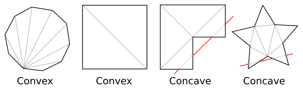
To know if a given polygon is concave or convex, it is rather easy. Convex polygons have all their diagonals contained inside, while it is not true for concave polygons, i.e. you can find two summits such that when you connect them, the segment is outside the polygon. Another test is to find a straight line that cross a concave polygon at more than two points as shown on the figure above with the red lines.
Convex polygons
For convex polygons, we have to consider two cases:
- points are ordered and describe the contour of the polygon
- points are unordered and spread randomly onto the 2d plane
For the second case, we can use scipy to compute the convex hull of the points such as to be in the first case situation:
import numpy as np
import scipy.spatial

P = np.random.uniform(-1.0, 1.0, (100,2))
P = P[scipy.spatial.ConvexHull(P).vertices]
From this ordered set of vertices describing the contour, it is now easy to
render the polygon using the gl.GL_TRIANGLE_FAN primitives:
@window.event
def on_draw(dt):
    window.clear()
    polygon.draw(gl.GL_TRIANGLE_FAN)
You can see on the figures below that it is better to use only the convex hull points to compute the triangulation. You can also check that all other points are actually inside the polygon area.
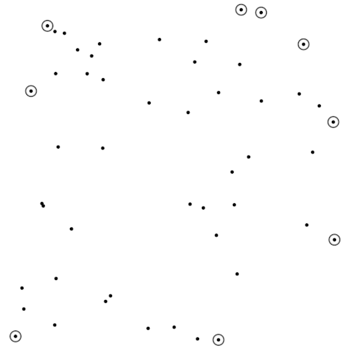
Figure
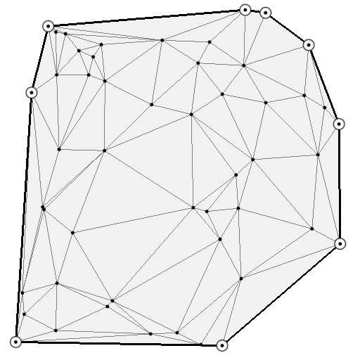
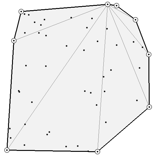
Concave polygons
For concave polygons, we could consider the two aforementionned cases where points are either ordered and describe the contour of the polygon or points are unordered and spread randomly onto the 2d plane. However, for the latter case, things become more difficult because the solution is not unique as shown on the figure below.
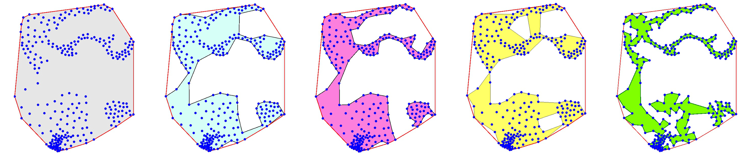
This is the reason why we'll restrict ourselves to the first case, that is, we have a set or ordered points describing the contour of a concave polygon. But even in such simple case, triangulation is not obvious and we'll thus need a dedicated library. We'll use the triangles library but there are others:
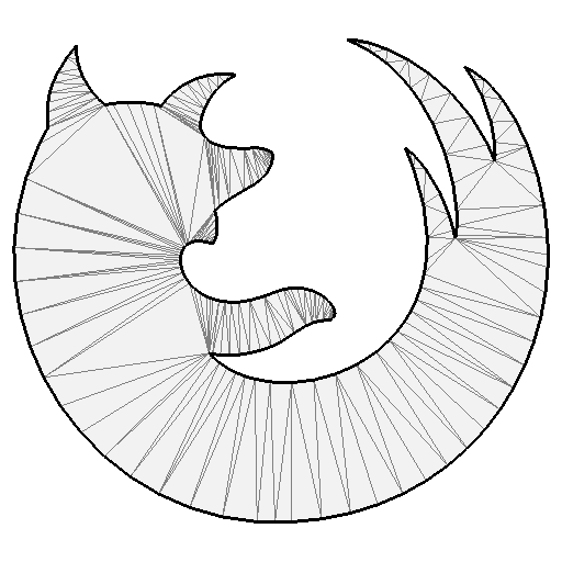
Figure
def triangulate(vertices):
    n = len(vertices)
    segments = (np.repeat(np.arange(n+1),2)[1:-1]) % n
    T = triangle.triangulate({'vertices': vertices,
                              'segments': segments}, "p")
    return T["vertices"], T["triangles"]
On the image on the right, we've parsed (see svg.py) the firefox icon SVG path and tesselated the Bézier
curves into line segments. Then we have triangulated the resulting path and
obtained the displayed triangulation using gl.GL_TRIANGLES. See firefox.py
Fill rule
The fill-rule property is used to specify how to paint the different parts of a shape. As explained in the SVG specification, for a simple, non-intersecting path, it is intuitively clear what region lies "inside"; however, for a more complex path, such as a path that intersects itself or where one subpath encloses another, the interpretation of "inside" is not so obvious. The fill-rule property provides two options for how the inside of a shape is determined: non-zero and even-odd.
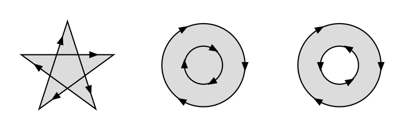
Figure
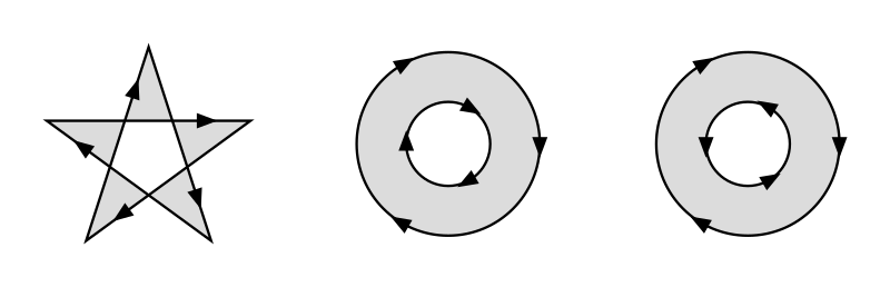
Figure
To enforce the fill-rule property, we'll need to use the stencil buffer that allows to have per-sample operation and test performed after the fragment shader stage. Depending on the stencil function and stencil operation we'll define, we can control precisely how a shape is rendered. But first, we need to tell OpenGL we'll be using a stencil buffer. In glumpy, the default is to have no stencil buffer, that is, the default bit depth of the stencil buffer is zero. To activate it, we thus simply need to specify some non-zero stencil bit depth (e.g. 8 for 256 possible values):
config = app.configuration.Configuration()
config.stencil_size = 8
window = app.Window(config=config, width=512, height=512)

@window.event
def on_init():
    gl.glEnable(gl.GL_STENCIL_TEST)
Note that we also need to activate the stencil test in the on_init window event.
Non-zero fill rule
The non-zero fill rule implementation is easy because it corresponds to the default triangulation we've just seen above and no extra work is necessary.
Odd-even fill rule
In order to enforce the odd-even fill rule, we need to use a 2-pass rendering. The first pass will write to the stencil buffer according to the operation we define and the second pass will read the stencil buffer in order to decide if a fragment need to be painted or not. For the first pass, we thus disable depth and color writing and we instruct OpenGL to increment stencil value if a shape is drawn clockwise (CW) and to decrement it for counter clock wise shapes (CCW):
# Disable color and depth writing
gl.glColorMask(gl.GL_FALSE, gl.GL_FALSE, gl.GL_FALSE, gl.GL_FALSE)
gl.glDepthMask(gl.GL_FALSE)

# Always write to stencil
gl.glStencilFunc(gl.GL_ALWAYS, 0, 0)

# Increment value for CW shape
gl.glStencilOpSeparate(gl.GL_FRONT, gl.GL_KEEP, gl.GL_KEEP, gl.GL_INCR)

# Decrement value for CCW shape
gl.glStencilOpSeparate(gl.GL_BACK,  gl.GL_KEEP, gl.GL_KEEP, gl.GL_DECR)
Once the stencil buffer has been written, we can use the stored value to decide
for the condition to be tested for writing to the render buffer. Using the
glStencilFunc function, we can express virtually any condition we want:
glStencilFunc(func, ref, mask)GL_NEVERAlways fails GL_LESSPasses if ( ref & mask ) < ( stencil & mask ) GL_LEQUALPasses if ( ref & mask ) <= ( stencil & mask ) GL_GREATERPasses if ( ref & mask ) > ( stencil & mask ) GL_GEQUALPasses if ( ref & mask ) >= ( stencil & mask ) GL_EQUALPasses if ( ref & mask ) = ( stencil & mask ) GL_NOTEQUALPasses if ( ref & mask ) != ( stencil & mask ) GL_ALWAYSAlways passes

For the actual odd-even fill rule, we only need to test for the last bit in the stencil buffer:
# Enable color and depth writing
gl.glColorMask(gl.GL_TRUE, gl.GL_TRUE, gl.GL_TRUE, gl.GL_TRUE)
gl.glDepthMask(gl.GL_TRUE)

# Actual stencil test
# Odd-even
gl.glStencilFunc(gl.GL_EQUAL, 0x01, 0x1)

# Non zero
# gl.glStencilFunc(gl.GL_NOTEQUAL, 0x00, 0xff)

# Positive
# gl.glStencilFunc(gl.GL_LESS, 0x0, 0xff)

# Stencil operation (for both CW and CCW shapes)
gl.glStencilOp(gl.GL_KEEP, gl.GL_KEEP, gl.GL_KEEP)
Exercises
Polygon gradients
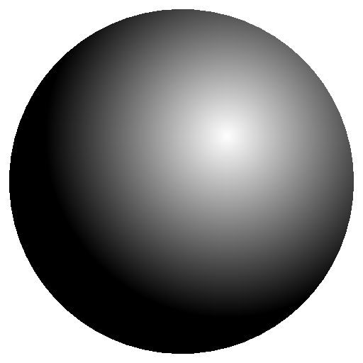
Figure
The SVG specification considers two kind of color gradients (i.e. smooth transition from one color to another), radial and linear. Using the vertices coordinates inside the shader, it is thus very easy to create those gradients. In order to do that, you need to compute (for every fragment) a scalar that indicate tells the amount of color 1 and color 2 respectively and try to render the image on the right.
Solution: radial-gradient.py
Polygon Patterns
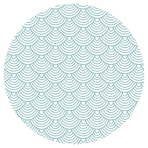
Figure
We can also use any texture to pain the polygon. It's only a matter of assigning the right texture to polygon vertices. Try to render the image on the right using this texture
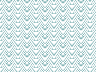
Solution: pattern.py
Antialiasing
As you have noticed, the polygon we've renderered so far are not antialised (because we've been using only raw triangles). While it might be possible to write a specific shader to take car of antiliasing on the border, it is far more easier to draw an antialiased polygon in two steps. First, we draw the interio of the polygon and then, we render a half-line on the contour. We need a half-line because we do not want the line to cover the already rendered polygon. There is no real difficulty and this is a good exercise. I will use the best proposed solution to be included here.
Rendering a mesh
Work in Progress.
Rendering text
Work in Progress.
Framebuffer
Work in Progress.
Special techniques
Work in Progress.
Conclusion
Work in Progress.
GLSL References
The information below has been directly extracted and reformated from the GLES Shading language 1.0. Copyright (c) 2006-2009 The Khronos Group Inc. All Rights Reserved. The teaser image above has been coded by Shadertoy Grand Master Íñigo Quílez and is available from the shadertoy website which is a great resource for learning OpenGL and WebGL (and that is more or less compatible with GLES 2.0).
Types
Scalar
void
for functions that do not return a value
bool
a conditional type, taking on values of true or false
int
a signed integer
float
a single floating-point scalar
Vector
bvec2 bvec3 bvec4
a two, three or four components Boolean vector
ivec2 ivec3 ivec4
a two, three or four components interge vector
vec2 vec3 vec4
a two, three or four components floating-point vector
Texture
sampler2D
a handle for accessing a 2D texture
samplerCube
a handle for accessing a cube mapped texture
Qualifiers
Storage
<none: default>
local read/write memory, or an input parameter to a function
const
a compile-time constant, or a function parameter that is read-only
attribute
linkage between a vertex shader and OpenGL ES for per-vertex data
uniform
value does not change across the primitive being processed, uniforms form the linkage between a shader, OpenGL ES, and the application
varying
linkage between a vertex shader and a fragment shader for interpolated data
Parameters
<none: default>
same as in
in
for function parameters passed into a function
out
for function parameters passed back out of a function, but not initialized for use when passed in
inout
for function parameters passed both into and out of a function
Precision
highp
Satisfies the minimum requirements for the vertex language. Optional in the fragment language.
mediump
Satisfies the minimum requirements for the fragment language. Its range and precision has to be greater than or the same as provided bylowpand less than or the same as provided byhighp.
lowp
Range and precision that can be less than mediump, but still intended to
represent all color values for any color channel.
Built-in variables
Vertex shader
These built-in vertex shader variables for communicating with fixed functionality are intrinsically declared with the following types:
highp   vec4  gl_Position;    // should be written to
mediump float gl_PointSize;   // may be written to
gl_Position
The variable gl_Position is intended for writing the homogeneous vertex
position.
gl_PointSize
The variable gl_PointSize is intended for a vertex shader to write the size
of the point to be rasterized. It is measured in pixels.
Fragment shader
The built-in variables that are accessible from a fragment shader are intrinsically given types as follows:
mediump vec4  gl_FragCoord;
        bool  gl_FrontFacing;
mediump vec4  gl_FragColor;
mediump vec4  gl_FragData[gl_MaxDrawBuffers];
mediump vec2  gl_PointCoord;
gl_FragColor
Writing to gl_FragColor specifies the fragment color that will be used by
the subsequent fixed functionality pipeline.
gl_FragData
gl_FragDatais an array. Writing togl_FragData[n]specifies the fragment data that will be used by the subsequent fixed functionality pipeline for data n.
gl_FragCoord
The variable gl_FragCoord is available as a read-only variable from within
fragment shaders and it holds the window relative coordinates x, y, z, and
1/w values for the fragment.
gl_FrontFacing
gl_FrontFacing value is true if the fragment belongs to a front-facing
primitive.
gl_PointCoord
The values in gl_PointCoord are two-dimensional coordinates indicating
where within a point primitive the current fragment is located. They range
from 0.0 to 1.0 across the point.
Built-in constants
The following built-in constants are provided to the vertex and fragment shaders. The example values below are the minimum values allowed for these maximums.
const mediump int gl_MaxVertexAttribs = 8;
const mediump int gl_MaxVertexUniformVectors = 128;
const mediump int gl_MaxVaryingVectors = 8;
const mediump int gl_MaxVertexTextureImageUnits = 0;
const mediump int gl_MaxCombinedTextureImageUnits = 8;
const mediump int gl_MaxTextureImageUnits = 8;
const mediump int gl_MaxFragmentUniformVectors = 16;
const mediump int gl_MaxDrawBuffers = 1;
Built-in functions
Angle and trigonometry functions
For all the functions below, T can be a float or a float vector (vec2,
vec3, vec4). In case of a float vector, the function is computed for each
component separately.
T radians (T degrees)
The
radiansfunction converts degrees to radians.float x = radians(90.0); // x = π/2 vec2 x = radians(vec2(45.0, 90.0)); // x = vec2(π/4, π/2)
T degrees (T radians)
The
degreefunction converts radians to degrees.const pi = 3.141592653589793; float x = degrees(pi); // x = 180 vec2 x = degrees(vec2(pi/4.0, pi/2.0)); // x = vec2(45.0, 90.0)
T sin (T angle)
The
sinfunction returns the sine of an angle in radians.const pi = 3.141592653589793; float x = sin(0.0); // x = 0 vec2 x = sin(vec2(0.0, pi/2.0)); // x = vec2(0.0, 1.0)
T cos (T angle)
The
cosfunction returns the cosine of an angle in radians.const pi = 3.141592653589793; float x = cos(0.0); // x = 0 vec2 x = cos(vec2(0.0, pi/2.0)); // x = vec2(1.0, 0.0)
T tan (T angle)
The
tanfunction returns the tangent of an angle in radians.const pi = 3.141592653589793; float x = tan(0.0); // x = 0 vec2 x = tan(vec2(0.0, pi/4.0)); // x = vec2(0.0, 1.0)
T asin (T x)
The
asinreturns an angle in radians whose sine is x. The range of values returned by this function is [−π/2,π/2] Results are undefined if ∣x∣ > 1.float x = asin(0.0); // x = 0.0 vec2 x = asin(vec2(0.0, 1.0)); // x = vec2(0.0, π/2)
T acos (T x)
The
acosreturns an angle in radians whose cosine is x. The range of values returned by this function is [0,π] Results are undefined if ∣x∣ > 1.float x = acos(0.0); // x = π/2 vec2 x = acos(vec2(0.0, 1.0)); // x = vec2(π/2, 0.0)
T atan (T y_over_x)
The
atanfunction returns an angle whose tangent is y/x. The signs of x and y are used to determine what quadrant the angle is in. The range of values returned by this function is [−π,π]. Results are undefined if x and y are both 0.float x = atan(0.0); // x = 0.0 vec2 x = atan(vec2(0.0, 1.0)); // x = vec2(0.0, π/4)
Exponential functions
For all the functions below, T can be a float or a float vector (vec2,
vec3, vec4). In case of a float vector, the function is computed for each
component separately.
T pow (T x, T y)
The
powerfunction returns x raised to the power of y, i.e., xʸ. Results are undefined if x < 0 or if x = 0 and y ≤ 0.float x = pow(2.0, 2.0); // x = 4.0 vec2 x = pow(vec2(2.0, 3.0), 2.0); // x = vec2(4.0, 9.0)
T exp (T x)
The
expfunction returns the natural exponentiation of x, i.e eˣ.float x = exp(2.0); // x = e² vec2 x = exp(vec2(2.0, 3.0)); // x = vec2(e², e³)
T log (T x)
The
logfunction returns the natural logarithm of x, i.e., returns the value y which satisfies the equation x = eʸ. Results are undefined if x ≤ 0.const float e = 2.718281828459045; float x = log(1.0); // x = 0.0 vec2 x = log(vec2(1.0, e)); // x = vec2(0.0, 1.0)
T exp2 (T x)
The
exp2function returns 2 raised to the x power, i.e., 2ˣfloat x = exp2(2.0); // x = 4.0 vec2 x = exp2(vec2(2.0, 3.0)); // x = vec2(4.0, 8.0)
T log2 (T x)
The
log2function returns the base 2 logarithm of x, i.e., returns the value y which satisfies the equation x = 2ʸ. Results are undefined if x ≤ 0.float x = log2(4.0); // x = 2.0 vec2 x = log2(vec2(4.0, 8.0)); // x = vec2(2.0, 3.0)
T sqrt (T x)
The
sqrtfunction returns the square root of x. Results are undefined if x < 0.float x = sqrt(4.0); // x = 2.0 vec2 x = sqrt(vec2(4.0, 9.0)); // x = vec2(2.0, 3.0)
T inversesqrt (T x)
The
inversesqrtreturns the inverse square root of x, i.e. the reciprocal of the square root. Results are undefined if x ≤ 0.float x = inversesqrt(1.0/4.0); // x = 2.0 vec2 x = sqrt(vec2(1.0/4.0, 1.0/9.0)); // x = vec2(2.0, 3.0)
Common functions
For all the functions below, T can be a float or a float vector (vec2,
vec3, vec4). In case of a float vector, the function is computed for each
component separately.
T abs (T x)
The
absfunction returns x if x ≥ 0, otherwise it returns –x.float x = abs(-1.0); // x = 1.0 vec2 x = abs(vec2(1.0, -2.0)); // x = vec2(1.0, 2.0)
T sign (T x)
The
signfunction returns 1.0 if x > 0, 0.0 if x = 0, and –1.0 if x < 0.float x = sign(-2.0); // x = -1.0 vec2 x = abs(vec2(0.0, 2.0)); // x = vec2(0.0, 1.0)
T floor (T x)
The
floorfunction returns a value equal to the nearest integer that is less than or equal to x.float x = sign(1.9); // x = 1.0 vec2 x = sign(vec2(-0.1, 1.1)); // x = vec2(-1.0, 1.0)
T ceil (T x)
The
ceilfunction returns a value equal to the nearest integer that is greater than or equal to x.float x = sign(1.9); // x = 2.0 vec2 x = sign(vec2(-0.1, 1.1)); // x = vec2(0.0, 2.0)
T fract (T x)
The
fracfunction returns the fractional part of x, i.e. x – floor (x).float x = frac(1.9); // x = 0.9 vec2 x = sign(vec2(-0.1, 1.1)); // x = vec2(0.9, 0.1)
T mod (T x, float y)
The
modfunction returns the modulus (modulo) of x, i.e. x – y * floor (x/y)float x = mod(1.1, 1.0); // x = 0.1 vec2 x = mod(vec2(1.1, 2.2), 1.0); // x = vec2(0.1, 0.2)
T mod (T x, T y)
The
modfunction returns the modulus (modulo) of x, i.e. x – y * floor (x/y).float x = mod(1.1, 1.0); // x = 0.1 vec2 x = mod(vec2(1.1, 2.2), vec2(1.0, 1.5)); // x = vec2(0.1, 0.7)
The
minfunction returns y if y < x, otherwise it returns xvec2 x = min(vec2(1.0, 2.0), vec2(0.0, 3.0)); // x = vec2(0.0, 2.0) vec2 x = min(vec2(1.0, 2.0), 1.0); // x = vec2(1.0, 1.0)
The
maxfunction returns y if x < y, otherwise it returns xvec2 x = max(vec2(1.0, 2.0), vec2(0.0, 3.0)); // x = vec2(1.0, 3.0) vec2 x = max(vec2(1.0, 2.0), 1.0); // x = vec2(1.0, 2.0)
The
clampfunction returnsmin(max(x,a),b). Results are undefined if a > b.float x = clamp(1.1, 0.0, 1.0); // x = 1.0; vec2 x = clamp(vec2(1.0, 2.0), 0.0, 1.0); // x = vec2(1.0, 1.0)
The
mixfunction returns the linear blend of x and y, i.e. x(1-a)+ya.float x = mix(0.0, 4.0, 0.25); // x = 1.0; float x = mix(0.0, 4.0, 0.75); // x = 3.0;
The
stepreturns 0.0 if x < edge, otherwise it returns 1.0float x = step(0.0, -1.0); // x = -1.0; float x = step(0.0, 0.5); // x = 1.0
The
smoothstepfunction returns 0.0 if x <= edge0 and 1.0 if x ≥ edge1 and performs smooth Hermite interpolation between 0 and 1 when edge0 < x < edge1. This is useful in cases where you would want a threshold function with a smooth transition. This is equivalent to:T t = clamp ((x – edge0) / (edge1 – edge0), 0, 1); return t * t * (3 – 2 * t);Results are undefined if edge0 >= edge1.
Geometric functions
float length (T x)
The
lengthfunction returns the length of vector x, i.e. the square root of the sum of the squares components.float x = length(1.0); // x = 1.0 float x = length(vec2(3.0,4.0)); // x = 5.0
float distance (T p0, T p1)
Returns the distance between p0 and p1, i.e.
length(p1-p0).vec3 p0 = vec3(1.0, 5.0, 7.0); vec3 p1 = vec3(1.0, 2.0, 3.0); float x = length(p0,p1); // x = 5.0
float dot (T x, T y)
Returns the dot product of x and y
vec3 cross (vec3 x, vec3 y)
The cross functionn returns the cross product of x and y.
T normalize (T x)
The
normalizefunction returns a vector in the same direction as x but with a length of 1.vec2 p = normalize(vec2(3.0, 4.0)); // x = vec2(3.0,4.0)/5.0
T faceforward(T N, T I,T Nref)
Thefaceforwardfunction return N ifdot(Nref, I) < 0, otherwise it returns –N.
T reflect (T I, T N)
For the incident vector I and surface orientation N, the reflect function
returns the reflection direction: I – 2 ∗ dot(N, I) ∗ N N must already be
normalized in order to achieve the desired result.
T refract (T I, T N, float eta)
For the incident vector I and surface normal N, and the ratio of indices of refraction eta, the
reftactfunction returns the refraction vector. The result is computed by:k = 1.0-eta*eta*(1.0-dot(N,I)*dot(N,I)) if (k < 0.0) return T(0) return eta*I-(eta*dot(N,I)+sqrt(k))*NThe input parameters for the incident vector I and the surface normal N must already be normalized to get the desired results.
Matrix functions
mat matrixCompMult (mat x, mat y)
The
matrixCompMultmultiply matrix x by matrix y component-wise, i.e.,result[i][j]is the scalar product ofx[i][j]andy[i][j].Note: to get linear algebraic matrix multiplication, use the multiply operator (*).
mat4 x = mat4(1.0);
mat4 y = mat4(2.0);
mat4 z = matrix CompMult(x,y); // z = mat4(2.0);
Vector Relational Functions
Relational and equality operators (<, <=, >, >=, ==, !=) are defined to produce
scalar Boolean results. For vector results, use the following built-in
functions. Below, bvecN is a placeholder for one of bvec2, bvec3, or
bvec4, ivecN is a placeholder for one of ivec2, ivec3, or ivec4, and
vecN is a placeholder for vec2, vec3, or vec4. In all cases, the sizes
of the input and return vectors for any particular call must match.
The
lessThanfunction returns the component-wise compare of x < y.bvec2 c = lessThan(vec2(1.0,1.0), vec2(1.0,2.0)); // x = vec2(false, true);
The
lessThanfunction returns the component-wise compare of x ≤ y.bvec2 c = lessThan(vec2(1.0,1.0), vec2(1.0,2.0)); // x = vec2(true, true);
The
greaterThanfunction returns the component-wise compare of x > y.bvec2 c = greaterThan(vec2(1.0,1.0), vec2(1.0,2.0)); // x = vec2(false, false);
The
greaterThanfunction returns the component-wise compare of x ≥ y.bvec2 c = greaterThan(vec2(1.0,1.0), vec2(1.0,2.0)); // x = vec2(true, false);
The
equalfunction returns the component-wise compare of x == y.ivec2 c = equald(ivec2(1,1), ivec2(1,2)); // x = vec2(true, false);
The
notEqualfunction returns the component-wise compare of x == y.ivec2 c = notEqual(ivec2(1,1), ovec2(1,2)); // x = vec2(false, true);
bool any (bvecN x)
The
anyfunction returns true if any component of x is true.bool x = any(bvec3(true, false, false)); // x = true bool x = any(bvec3(false, false, false)); // x = false
bool all (bvecN x)
The
allfunction returns true only if all components of x are true.bool x = all(bvec3(true, true, true)); // x = true bool x = all(bvec3(true, true, false)); // x = false
bvecN not (bvecN x)
Returns the component-wise logical complement of x.
bvec2 x = not(bvec2(true, false)); // x = bvec2(false, true)
Texture lookup functions
vec4 texture2D (sampler2D sampler, vec2 coord)
Use the texture coordinate coord to do a texture lookup in the 2D texture currently bound to sampler.
vec4 textureCube (samplerCube sampler, vec3 coord )
Use the texture coordinate coord to do a texture lookup in the cube map texture currently bound to sampler. The direction of coord is used to select which face to do a 2- dimensional texture lookup in, as described in section 3.8.6 in version 2.0 of the OpenGL specification.
Bibliography
This is a curated list of some computer graphics resources (peoole, articles, books & tutorials) addressing different aspects. Some are very specific to OpenGL while some others offer a broader view on computer graphics and geometry.
People
- Íñigo Quílez wrote short articles on the techniques he developed for computer graphics experiments, demos, shadertoys and movies. All content is beginner and medium level, and mostly pragmatic rather than theoretical. He is also a master in raymarched distance fields and wrote some of the most amazing scripts on shadertoys (see for example his beautiful snail script.
- Paul Bourke offers on his website a very large set of resources concerning Geometry, Surfaces, Curves & Polyhedra (among other things). He generally get straight to the point with demonstration and code. I cannot count the number of times I landed on his page when asking a simple geometry questions (distance between two lines in 3D, circles passing through three points, intersecion of two circles, etc).
- Philip Rideout maintains the Little Grasshoper website where he explains some specific techniques such as volumetric smoke, tesselation, clipping). Everything comes with code, demos and explanations and I translated some of his techniques in this book.
Tutorials
- Open GL tutorial (C), Sam Hocevar, 2017.
- Learn OpenGL (C), Joey de Vries, 2017.
- An intro to modern OpenGL (C), Joe Groff, 2010.
- OpenGL Wiki, Community Edited, 2017.
- Fundamental OpenGL tutorial, Song Ho Ahn (안성호), 2017.
- Tiny renderer, Dmitry V. Sokolov, 2016.
Articles
- N. P. Rougier, Journal of Computer Graphics Techniques (JCGT), vol. 2, no. 1, pp. 50–64, 2013.
Even though text is pervasive in most 3D applications, there is surprisingly no native support for text rendering in OpenGL. To cope with this absence, Mark Kilgard introduced the use of texture fonts [Kilgard 1997]. This technique is well known and widely used and ensures both good performances and a decent quality in most situations. However, the quality may degrade strongly in orthographic mode (screen space) due to pixelation effects at large sizes and to legibility problems at small sizes due to incorrect hinting and positioning of glyphs. In this paper, we consider font-texture rendering to develop methods to ensure the highest quality in orthographic mode. The method used allows for both the accurate render- ing and positioning of any glyph on the screen. While the method is compatible with complex shaping and/or layout (e.g., the Arabic alphabet), these specific cases are not studied in this article.
- N. P. Rougier Journal of Computer Graphics Techniques (JCGT), vol. 2, no. 2, pp. 105–121, 2013.
Dashed stroked paths are a widely-used feature found in the vast majority of vector-drawing software and libraries. They enable, for example, the highlighting of a given path, such as the current selection, in drawing software or distinguishing curves, in the case of a scientific plotting package. This paper introduces a shader-based method for rendering arbitrary dash patterns along any continuous polyline (smooth or broken). The proposed method does not tessellate individual dash patterns and allows for fast and nearly accurate rendering of any user-defined dash pattern and caps. Benchmarks indicate a slowdown ratio between 1.1 and 2.1 with an increased memory consumption between 3 and 6. Furthermore, the method can be used for solid thick polylines with correct caps and joins with only a slowdown factor of 1.1.
- N. P. Rougier Journal of Computer Graphics Techniques (JCGT), vol. 3, no. 4, pp. 1–52, 2014.
Grids, markers, and arrows are important components in scientific visualisation. Grids are widely used in scientific plots and help visually locate data. Markers visualize individual points and aggregated data. Quiver plots show vector fields, such as a velocity buffer, through regularly-placed arrows. Being able to draw these components quickly is critical if one wants to offer interactive visualisation. This article provides algorithms with GLSL implementations for drawing grids, markers, and arrows using implicit surfaces that make it possible quickly render pixel-perfect antialiased shapes.
Books
- Morgan McGuire, 2017.
The Graphics Codex is designed to support a course either as the sole, standalone text or as lecture notes and an encyclopedic reference alongside a traditional textbook. It contains 400 cross-referenced equation and diagram entries, 14 chapters on physically-based shading and rendering Multi-platform programming projects, Links to external DirectX, OpenGL, Unity, Mitsuba, G3D, and other API documentation, PDF links and full citations for primary sources and textbooks, Free updates with new content every month
- Tomas Akenine-Moller, Eric Haines, Naty Hoffman
Thoroughly revised, this third edition focuses on modern techniques used to generate synthetic three-dimensional images in a fraction of a second. With the advent of programmable shaders, a wide variety of new algorithms have arisen and evolved over the past few years. This edition discusses current, practical rendering methods used in games and other applications. It also presents a solid theoretical framework and relevant mathematics for the field of interactive computer graphics, all in an approachable style.
- John F. Hughes, Andries van Dam, Morgan McGuire, David F. Sklar, James D. Foley, Steven K. Feiner, Kurt Akeley
In this book, we explain the principles, as well as the mathematics, underlying computer graphics--knowledge that is essential for successful work both now and in the future. Early chapters show how to create 2D and 3D pictures right away, supporting experimentation. Later chapters, covering a broad range of topics, demonstrate more sophisticated approaches. Sections on current computer graphics practice show how to apply given principles in common situations, such as how to approximate an ideal solution on available hardware, or how to represent a data structure more efficiently. Topics are reinforced by exercises, programming problems, and hands-on projects.
- Peter Shirley, Michael Ashikhmin, Steve Marschner
The third edition of this widely adopted text gives students a comprehensive, fundamental introduction to computer graphics. The authors present the mathematical foundations of computer graphics with a focus on geometric intuition, allowing the programmer to understand and apply those foundations to the development of efficient code.
- Nicolas P. Rougier
There are already a fair number of books about Numpy and a legitimate question is to wonder if another book is really necessary. As you may have guessed by reading these lines, my personal answer is yes, mostly because I think there is room for a different approach concentrating on the migration from Python to Numpy through vectorization. There are a lot of techniques that you don't find in books and such techniques are mostly learned through experience. The goal of this book is to explain some of these techniques and to provide an opportunity for making this experience in the process.